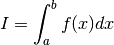
Numerical integration (quadrature)
Standard quadrature (quad)
- mpmath.quad(ctx, f, *points, **kwargs)
Computes a single, double or triple integral over a given 1D interval, 2D rectangle, or 3D cuboid. A basic example:
>>> from mpmath import *
>>> mp.dps = 15; mp.pretty = True
>>> quad(sin, [0, pi])
2.0
A basic 2D integral:
>>> f = lambda x, y: cos(x+y/2)
>>> quad(f, [-pi/2, pi/2], [0, pi])
4.0
Interval format
The integration range for each dimension may be specified using a list or tuple. Arguments are interpreted as follows:
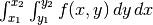
quad(f, [x1, x2]) – calculates

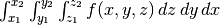
quad(f, [x1, x2], [y1, y2]) – calculates
quad(f, [x1, x2], [y1, y2], [z1, z2]) – calculates
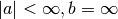
Endpoints may be finite or infinite. An interval descriptor may also contain more than two points. In this case, the integration is split into subintervals, between each pair of consecutive points. This is useful for dealing with mid-interval discontinuities, or integrating over large intervals where the function is irregular or oscillates.
Options
quad() recognizes the following keyword arguments:
- method
- Chooses integration algorithm (described below).
- error
- If set to true, quad() returns
 where
where  is the
integral and
is the
integral and  is the estimated error.
 - maxdegree
- Maximum degree of the quadrature rule to try before quitting.
- verbose
- Print details about progress.
Algorithms
Mpmath presently implements two integration algorithms: tanh-sinh quadrature and Gauss-Legendre quadrature. These can be selected using method=’tanh-sinh’ or method=’gauss-legendre’ or by passing the classes method=TanhSinh, method=GaussLegendre. The functions quadts() and quadgl() are also available as shortcuts.
Both algorithms have the property that doubling the number of evaluation points roughly doubles the accuracy, so both are ideal for high precision quadrature (hundreds or thousands of digits).
At high precision, computing the nodes and weights for the integration can be expensive (more expensive than computing the function values). To make repeated integrations fast, nodes are automatically cached.
The advantages of the tanh-sinh algorithm are that it tends to handle endpoint singularities well, and that the nodes are cheap to compute on the first run. For these reasons, it is used by quad() as the default algorithm.
Gauss-Legendre quadrature often requires fewer function evaluations, and is therefore often faster for repeated use, but the algorithm does not handle endpoint singularities as well and the nodes are more expensive to compute. Gauss-Legendre quadrature can be a better choice if the integrand is smooth and repeated integrations are required (e.g. for multiple integrals).
See the documentation for TanhSinh and GaussLegendre for additional details.
Examples of 1D integrals
Intervals may be infinite or half-infinite. The following two examples evaluate the limits of the inverse tangent function (
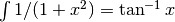 ), and the Gaussian integral
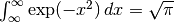 :
:>>> mp.dps = 15 >>> quad(lambda x: 2/(x**2+1), [0, inf]) 3.14159265358979 >>> quad(lambda x: exp(-x**2), [-inf, inf])**2 3.14159265358979
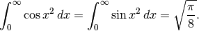
Integrals can typically be resolved to high precision. The following computes 50 digits of
 by integrating the
area of the half-circle defined by
by integrating the
area of the half-circle defined by  ,
,
 ,
,  :
:>>> mp.dps = 50 >>> 2*quad(lambda x: sqrt(1-x**2), [-1, 1]) 3.1415926535897932384626433832795028841971693993751
One can just as well compute 1000 digits (output truncated):
>>> mp.dps = 1000
>>> 2*quad(lambda x: sqrt(1-x**2), [-1, 1])
3.141592653589793238462643383279502884...216420198
Complex integrals are supported. The following computes a residue at
 by integrating counterclockwise along the
diamond-shaped path from
by integrating counterclockwise along the
diamond-shaped path from  to
to  to
to  to
to  to :
to :>>> mp.dps = 15 >>> chop(quad(lambda z: 1/z, [1,j,-1,-j,1])) (0.0 + 6.28318530717959j)
Examples of 2D and 3D integrals
Here are several nice examples of analytically solvable 2D integrals (taken from MathWorld [1]) that can be evaluated to high precision fairly rapidly by quad():
>>> mp.dps = 30
>>> f = lambda x, y: (x-1)/((1-x*y)*log(x*y))
>>> quad(f, [0, 1], [0, 1])
0.577215664901532860606512090082
>>> +euler
0.577215664901532860606512090082

>>> f = lambda x, y: 1/sqrt(1+x**2+y**2)
>>> quad(f, [-1, 1], [-1, 1])
3.17343648530607134219175646705
>>> 4*log(2+sqrt(3))-2*pi/3
3.17343648530607134219175646705

>>> f = lambda x, y: 1/(1-x**2 * y**2)
>>> quad(f, [0, 1], [0, 1])
1.23370055013616982735431137498
>>> pi**2 / 8
1.23370055013616982735431137498

>>> quad(lambda x, y: 1/(1-x*y), [0, 1], [0, 1])
1.64493406684822643647241516665
>>> pi**2 / 6
1.64493406684822643647241516665
Multiple integrals may be done over infinite ranges:
>>> mp.dps = 15
>>> print(quad(lambda x,y: exp(-x-y), [0, inf], [1, inf]))
0.367879441171442
>>> print(1/e)
0.367879441171442
For nonrectangular areas, one can call quad() recursively. For example, we can replicate the earlier example of calculating
by integrating over the unit-circle, and actually use double
quadrature to actually measure the area circle:>>> f = lambda x: quad(lambda y: 1, [-sqrt(1-x**2), sqrt(1-x**2)]) >>> quad(f, [-1, 1]) 3.14159265358979
Here is a simple triple integral:
>>> mp.dps = 15
>>> f = lambda x,y,z: x*y/(1+z)
>>> quad(f, [0,1], [0,1], [1,2], method='gauss-legendre')
0.101366277027041
>>> (log(3)-log(2))/4
0.101366277027041
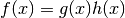
Singularities
Both tanh-sinh and Gauss-Legendre quadrature are designed to integrate smooth (infinitely differentiable) functions. Neither algorithm copes well with mid-interval singularities (such as mid-interval discontinuities in
 or
or  ).
The best solution is to split the integral into parts:
).
The best solution is to split the integral into parts:>>> mp.dps = 15 >>> quad(lambda x: abs(sin(x)), [0, 2*pi]) # Bad 3.99900894176779 >>> quad(lambda x: abs(sin(x)), [0, pi, 2*pi]) # Good 4.0
The tanh-sinh rule often works well for integrands having a singularity at one or both endpoints:
>>> mp.dps = 15
>>> quad(log, [0, 1], method='tanh-sinh')  # Good
-1.0
>>> quad(log, [0, 1], method='gauss-legendre')  # Bad
-0.999932197413801
However, the result may still be inaccurate for some functions:
>>> quad(lambda x: 1/sqrt(x), [0, 1], method='tanh-sinh')
1.99999999946942
This problem is not due to the quadrature rule per se, but to numerical amplification of errors in the nodes. The problem can be circumvented by temporarily increasing the precision:
>>> mp.dps = 30
>>> a = quad(lambda x: 1/sqrt(x), [0, 1], method='tanh-sinh')
>>> mp.dps = 15
>>> +a
2.0
Highly variable functions
For functions that are smooth (in the sense of being infinitely differentiable) but contain sharp mid-interval peaks or many “bumps”, quad() may fail to provide full accuracy. For example, with default settings, quad() is able to integrate
 accurately over an interval of length 100 but not over
length 1000:
accurately over an interval of length 100 but not over
length 1000:>>> quad(sin, [0, 100]); 1-cos(100) # Good 0.137681127712316 0.137681127712316 >>> quad(sin, [0, 1000]); 1-cos(1000) # Bad -37.8587612408485 0.437620923709297
One solution is to break the integration into 10 intervals of length 100:
>>> quad(sin, linspace(0, 1000, 10))   # Good
0.437620923709297
Another is to increase the degree of the quadrature:
>>> quad(sin, [0, 1000], maxdegree=10)   # Also good
0.437620923709297
Whether splitting the interval or increasing the degree is more efficient differs from case to case. Another example is the function
 , which has a sharp peak centered around
 :
:>>> f = lambda x: 1/(1+x**2) >>> quad(f, [-100, 100]) # Bad 3.64804647105268 >>> quad(f, [-100, 100], maxdegree=10) # Good 3.12159332021646 >>> quad(f, [-100, 0, 100]) # Also good 3.12159332021646
References
Oscillatory quadrature (quadosc)
- mpmath.quadosc(ctx, f, interval, omega=None, period=None, zeros=None)
Calculates
where at least one of
 and
and  is infinite and where
 for some slowly
decreasing function
for some slowly
decreasing function  . With proper input, quadosc()
can also handle oscillatory integrals where the oscillation
rate is different from a pure sine or cosine wave.
. With proper input, quadosc()
can also handle oscillatory integrals where the oscillation
rate is different from a pure sine or cosine wave.In the standard case when
 ,
quadosc() works by evaluating the infinite series
,
quadosc() works by evaluating the infinite series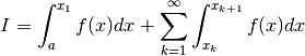
where
 are consecutive zeros (alternatively
some other periodic reference point) of .
Accordingly, quadosc() requires information about the
zeros of . For a periodic function, you can specify
the zeros by either providing the angular frequency
are consecutive zeros (alternatively
some other periodic reference point) of .
Accordingly, quadosc() requires information about the
zeros of . For a periodic function, you can specify
the zeros by either providing the angular frequency  (omega) or the period
  . In general, you can
specify the
. In general, you can
specify the  -th zero by providing the zeros arguments.
Below is an example of each:
-th zero by providing the zeros arguments.
Below is an example of each:>>> from mpmath import * >>> mp.dps = 15; mp.pretty = True >>> f = lambda x: sin(3*x)/(x**2+1) >>> quadosc(f, [0,inf], omega=3) 0.37833007080198 >>> quadosc(f, [0,inf], period=2*pi/3) 0.37833007080198 >>> quadosc(f, [0,inf], zeros=lambda n: pi*n/3) 0.37833007080198 >>> (ei(3)*exp(-3)-exp(3)*ei(-3))/2 # Computed by Mathematica 0.37833007080198
Note that zeros was specified to multiply
by the
half-period, not the full period. In theory, it does not matter
whether each partial integral is done over a half period or a full
period. However, if done over half-periods, the infinite series
passed to nsum() becomes an alternating series and this
typically makes the extrapolation much more efficient.Here is an example of an integration over the entire real line, and a half-infinite integration starting at
 :
:>>> quadosc(lambda x: cos(x)/(1+x**2), [-inf, inf], omega=1) 1.15572734979092 >>> pi/e 1.15572734979092 >>> quadosc(lambda x: cos(x)/x**2, [-inf, -1], period=2*pi) -0.0844109505595739 >>> cos(1)+si(1)-pi/2 -0.0844109505595738
Of course, the integrand may contain a complex exponential just as well as a real sine or cosine:
>>> quadosc(lambda x: exp(3*j*x)/(1+x**2), [-inf,inf], omega=3)
(0.156410688228254 + 0.0j)
>>> pi/e**3
0.156410688228254
>>> quadosc(lambda x: exp(3*j*x)/(2+x+x**2), [-inf,inf], omega=3)
(0.00317486988463794 - 0.0447701735209082j)
>>> 2*pi/sqrt(7)/exp(3*(j+sqrt(7))/2)
(0.00317486988463794 - 0.0447701735209082j)
Non-periodic functions
If
 for some function
  that is not
strictly periodic, omega or period might not work, and it might
be necessary to use zeros.
that is not
strictly periodic, omega or period might not work, and it might
be necessary to use zeros.A notable exception can be made for Bessel functions which, though not periodic, are “asymptotically periodic” in a sufficiently strong sense that the sum extrapolation will work out:
>>> quadosc(j0, [0, inf], period=2*pi)
1.0
>>> quadosc(j1, [0, inf], period=2*pi)
1.0
More properly, one should provide the exact Bessel function zeros:
>>> j0zero = lambda n: findroot(j0, pi*(n-0.25))
>>> quadosc(j0, [0, inf], zeros=j0zero)
1.0
For an example where zeros becomes necessary, consider the complete Fresnel integrals
Although the integrands do not decrease in magnitude as
 , the integrals are convergent since the oscillation
rate increases (causing consecutive periods to asymptotically
cancel out). These integrals are virtually impossible to calculate
to any kind of accuracy using standard quadrature rules. However,
if one provides the correct asymptotic distribution of zeros
(
, the integrals are convergent since the oscillation
rate increases (causing consecutive periods to asymptotically
cancel out). These integrals are virtually impossible to calculate
to any kind of accuracy using standard quadrature rules. However,
if one provides the correct asymptotic distribution of zeros
( ), quadosc() works:
>>> mp.dps = 30
>>> f = lambda x: cos(x**2)
>>> quadosc(f, [0,inf], zeros=lambda n:sqrt(pi*n))
0.626657068657750125603941321203
>>> f = lambda x: sin(x**2)
>>> quadosc(f, [0,inf], zeros=lambda n:sqrt(pi*n))
0.626657068657750125603941321203
>>> sqrt(pi/8)
0.626657068657750125603941321203
(Interestingly, these integrals can still be evaluated if one places some other constant than
in the square root sign.)In general, if
 , the zeros follow
the inverse-function distribution
, the zeros follow
the inverse-function distribution  :
:>>> mp.dps = 15 >>> f = lambda x: sin(exp(x)) >>> quadosc(f, [1,inf], zeros=lambda n: log(n)) -0.25024394235267 >>> pi/2-si(e) -0.250243942352671
Non-alternating functions
If the integrand oscillates around a positive value, without alternating signs, the extrapolation might fail. A simple trick that sometimes works is to multiply or divide the frequency by 2:
>>> f = lambda x: 1/x**2+sin(x)/x**4
>>> quadosc(f, [1,inf], omega=1)  # Bad
1.28642190869861
>>> quadosc(f, [1,inf], omega=0.5)  # Perfect
1.28652953559617
>>> 1+(cos(1)+ci(1)+sin(1))/6
1.28652953559617
Fast decay
quadosc() is primarily useful for slowly decaying integrands. If the integrand decreases exponentially or faster, quad() will likely handle it without trouble (and generally be much faster than quadosc()):
>>> quadosc(lambda x: cos(x)/exp(x), [0, inf], omega=1)
0.5
>>> quad(lambda x: cos(x)/exp(x), [0, inf])
0.5
Quadrature rules
- class mpmath.calculus.quadrature.QuadratureRule(ctx)
Quadrature rules are implemented using this class, in order to simplify the code and provide a common infrastructure for tasks such as error estimation and node caching.
You can implement a custom quadrature rule by subclassing QuadratureRule and implementing the appropriate methods. The subclass can then be used by quad() by passing it as the method argument.
QuadratureRule instances are supposed to be singletons. QuadratureRule therefore implements instance caching in __new__().
- calc_nodes(degree, prec, verbose=False)
Compute nodes for the standard interval
![[-1, 1]](../_images/math/5c3818b9565a33fd3aadba10026d32c5e3eea90f.png) . Subclasses
should probably implement only this method, and use
get_nodes() method to retrieve the nodes.
. Subclasses
should probably implement only this method, and use
get_nodes() method to retrieve the nodes.
- clear()
Delete cached node data.
- estimate_error(results, prec, epsilon)
Given results from integrations
![[I_1, I_2, \ldots, I_k]](../_images/math/dbc47e6361fa8fb5c5677d7f82dfa0ee87591207.png) done
with a quadrature of rule of degree
done
with a quadrature of rule of degree  , estimate
the error of
, estimate
the error of  .
.For
 , we estimate
  as
as  .
.For
 , we extrapolate
  from
from  and
and  under the assumption
that each degree increment roughly doubles the accuracy of
the quadrature rule (this is true for both TanhSinh
and GaussLegendre). The extrapolation formula is given
by Borwein, Bailey & Girgensohn. Although not very conservative,
this method seems to be very robust in practice.
under the assumption
that each degree increment roughly doubles the accuracy of
the quadrature rule (this is true for both TanhSinh
and GaussLegendre). The extrapolation formula is given
by Borwein, Bailey & Girgensohn. Although not very conservative,
this method seems to be very robust in practice.
- get_nodes(a, b, degree, prec, verbose=False)
Return nodes for given interval, degree and precision. The nodes are retrieved from a cache if already computed; otherwise they are computed by calling calc_nodes() and are then cached.
Subclasses should probably not implement this method, but just implement calc_nodes() for the actual node computation.
- guess_degree(prec)
Given a desired precision
 in bits, estimate the degree
  of the quadrature required to accomplish full accuracy for
typical integrals. By default, quad() will perform up
to iterations. The value of should be a slight
overestimate, so that “slightly bad” integrals can be dealt
with automatically using a few extra iterations. On the
other hand, it should not be too big, so quad() can
quit within a reasonable amount of time when it is given
an “unsolvable” integral.
of the quadrature required to accomplish full accuracy for
typical integrals. By default, quad() will perform up
to iterations. The value of should be a slight
overestimate, so that “slightly bad” integrals can be dealt
with automatically using a few extra iterations. On the
other hand, it should not be too big, so quad() can
quit within a reasonable amount of time when it is given
an “unsolvable” integral.The default formula used by guess_degree() is tuned for both TanhSinh and GaussLegendre. The output is roughly as follows:
50 6 100 7 500 10 3000 12 This formula is based purely on a limited amount of experimentation and will sometimes be wrong.
- sum_next(f, nodes, degree, prec, previous, verbose=False)
Evaluates the step sum
 where the nodes list
contains the
where the nodes list
contains the  pairs.
summation() will supply the list results of values computed by sum_next() at previous degrees, in case the quadrature rule is able to reuse them.
- summation(f, points, prec, epsilon, max_degree, verbose=False)
Main integration function. Computes the 1D integral over the interval specified by points. For each subinterval, performs quadrature of degree from 1 up to max_degree until estimate_error() signals convergence.
summation() transforms each subintegration to the standard interval and then calls sum_next().
- transform_nodes(nodes, a, b, verbose=False)
Rescale standardized nodes (for
) to a general
interval ![[a, b]](../_images/math/da2e551d2ca2155b8d8f4935d2e9757722c9bab6.png) . For a finite interval, a simple linear
change of variables is used. Otherwise, the following
transformations are used:
. For a finite interval, a simple linear
change of variables is used. Otherwise, the following
transformations are used:![[a, \infty] : t = \frac{1}{x} + (a-1)
[-\infty, b] : t = (b+1) - \frac{1}{x}
[-\infty, \infty] : t = \frac{x}{\sqrt{1-x^2}}](../_images/math/733647b1ab0cd443827387b1e630fa38a826acf0.png)
Tanh-sinh rule
- class mpmath.calculus.quadrature.TanhSinh(ctx)
This class implements “tanh-sinh” or “doubly exponential” quadrature. This quadrature rule is based on the Euler-Maclaurin integral formula. By performing a change of variables involving nested exponentials / hyperbolic functions (hence the name), the derivatives at the endpoints vanish rapidly. Since the error term in the Euler-Maclaurin formula depends on the derivatives at the endpoints, a simple step sum becomes extremely accurate. In practice, this means that doubling the number of evaluation points roughly doubles the number of accurate digits.
- Comparison to Gauss-Legendre:
- Initial computation of nodes is usually faster
- Handles endpoint singularities better
- Handles infinite integration intervals better
- Is slower for smooth integrands once nodes have been computed
The implementation of the tanh-sinh algorithm is based on the description given in Borwein, Bailey & Girgensohn, “Experimentation in Mathematics - Computational Paths to Discovery”, A K Peters, 2003, pages 312-313. In the present implementation, a few improvements have been made:
- A more efficient scheme is used to compute nodes (exploiting recurrence for the exponential function)
- The nodes are computed successively instead of all at once
Various documents describing the algorithm are available online, e.g.:
- calc_nodes(degree, prec, verbose=False)
The abscissas and weights for tanh-sinh quadrature of degree
are given by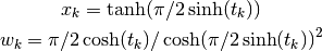
where
 for a step length
  . The
list of nodes is actually infinite, but the weights die off so
rapidly that only a few are needed.
. The
list of nodes is actually infinite, but the weights die off so
rapidly that only a few are needed.
- sum_next(f, nodes, degree, prec, previous, verbose=False)
Step sum for tanh-sinh quadrature of degree
. We exploit the
fact that half of the abscissas at degree are precisely the
abscissas from degree  . Thus reusing the result from
the previous level allows a 2x speedup.
. Thus reusing the result from
the previous level allows a 2x speedup.
Gauss-Legendre rule
- class mpmath.calculus.quadrature.GaussLegendre(ctx)
This class implements Gauss-Legendre quadrature, which is exceptionally efficient for polynomials and polynomial-like (i.e. very smooth) integrands.
The abscissas and weights are given by roots and values of Legendre polynomials, which are the orthogonal polynomials on
with respect to the unit weight
(see legendre()).In this implementation, we take the “degree”
of the quadrature
to denote a Gauss-Legendre rule of degree  (following
Borwein, Bailey & Girgensohn). This way we get quadratic, rather
than linear, convergence as the degree is incremented.
(following
Borwein, Bailey & Girgensohn). This way we get quadratic, rather
than linear, convergence as the degree is incremented.- Comparison to tanh-sinh quadrature:
- Is faster for smooth integrands once nodes have been computed
- Initial computation of nodes is usually slower
- Handles endpoint singularities worse
- Handles infinite integration intervals worse
- calc_nodes(degree, prec, verbose=False)
Calculates the abscissas and weights for Gauss-Legendre quadrature of degree of given degree (actually
).