Differentiation¶

Numerical derivatives (`diff`, `diffs`)¶

mpmath.diff(ctx, f, x, n=1, **options)¶

Numerically computes the derivative of $f$ , $f'(x)$ , or generally for an integer $n \ge 0$ , the $n$ -th derivative $f^{(n)}(x)$ . A few basic examples are:

>>> from mpmath import *
>>> mp.dps = 15; mp.pretty = True
>>> diff(lambda x: x**2 + x, 1.0)
3.0
>>> diff(lambda x: x**2 + x, 1.0, 2)
2.0
>>> diff(lambda x: x**2 + x, 1.0, 3)
0.0
>>> nprint([diff(exp, 3, n) for n in range(5)])   # exp'(x) = exp(x)
[20.0855, 20.0855, 20.0855, 20.0855, 20.0855]

Even more generally, given a tuple of arguments $(x_1, \ldots, x_k)$ and order $(n_1, \ldots, n_k)$ , the partial derivative $f^{(n_1,\ldots,n_k)}(x_1,\ldots,x_k)$ is evaluated. For example:

>>> diff(lambda x,y: 3*x*y + 2*y - x, (0.25, 0.5), (0,1))
2.75
>>> diff(lambda x,y: 3*x*y + 2*y - x, (0.25, 0.5), (1,1))
3.0

Options

The following optional keyword arguments are recognized:

method: Supported methods are 'step' or 'quad': derivatives may be computed using either a finite difference with a small step size $h$ (default), or numerical quadrature.
direction: Direction of finite difference: can be -1 for a left difference, 0 for a central difference (default), or +1 for a right difference; more generally can be any complex number.
addprec: Extra precision for $h$ used to account for the function’s sensitivity to perturbations (default = 10).
relative: Choose $h$ relative to the magnitude of $x$ , rather than an absolute value; useful for large or tiny $x$ (default = False).
h: As an alternative to addprec and relative, manually select the step size $h$ .
singular: If True, evaluation exactly at the point $x$ is avoided; this is useful for differentiating functions with removable singularities. Default = False.
radius: Radius of integration contour (with method = 'quad'). Default = 0.25. A larger radius typically is faster and more accurate, but it must be chosen so that $f$ has no singularities within the radius from the evaluation point.

A finite difference requires $n+1$ function evaluations and must be performed at $(n+1)$ times the target precision. Accordingly, $f$ must support fast evaluation at high precision.

With integration, a larger number of function evaluations is required, but not much extra precision is required. For high order derivatives, this method may thus be faster if f is very expensive to evaluate at high precision.

Further examples

The direction option is useful for computing left- or right-sided derivatives of nonsmooth functions:

>>> diff(abs, 0, direction=0)
0.0
>>> diff(abs, 0, direction=1)
1.0
>>> diff(abs, 0, direction=-1)
-1.0

More generally, if the direction is nonzero, a right difference is computed where the step size is multiplied by sign(direction). For example, with direction=+j, the derivative from the positive imaginary direction will be computed:

>>> diff(abs, 0, direction=j)
(0.0 - 1.0j)

With integration, the result may have a small imaginary part even even if the result is purely real:

>>> diff(sqrt, 1, method='quad')    
(0.5 - 4.59...e-26j)
>>> chop(_)
0.5

Adding precision to obtain an accurate value:

>>> diff(cos, 1e-30)
0.0
>>> diff(cos, 1e-30, h=0.0001)
-9.99999998328279e-31
>>> diff(cos, 1e-30, addprec=100)
-1.0e-30

mpmath.diffs(ctx, f, x, n=None, **options)¶

Returns a generator that yields the sequence of derivatives

$f(x), f'(x), f''(x), \ldots, f^{(k)}(x), \ldots$

With method='step', diffs() uses only $O(k)$ function evaluations to generate the first $k$ derivatives, rather than the roughly $O(k^2)$ evaluations required if one calls diff() $k$ separate times.

With $n < \infty$ , the generator stops as soon as the $n$ -th derivative has been generated. If the exact number of needed derivatives is known in advance, this is further slightly more efficient.

Options are the same as for diff().

Examples

>>> from mpmath import *
>>> mp.dps = 15
>>> nprint(list(diffs(cos, 1, 5)))
[0.540302, -0.841471, -0.540302, 0.841471, 0.540302, -0.841471]
>>> for i, d in zip(range(6), diffs(cos, 1)):
...     print("%s %s" % (i, d))
...
0 0.54030230586814
1 -0.841470984807897
2 -0.54030230586814
3 0.841470984807897
4 0.54030230586814
5 -0.841470984807897

Composition of derivatives (`diffs_prod`, `diffs_exp`)¶

mpmath.diffs_prod(ctx, factors)¶

Given a list of $N$ iterables or generators yielding $f_k(x), f'_k(x), f''_k(x), \ldots$ for $k = 1, \ldots, N$ , generate $g(x), g'(x), g''(x), \ldots$ where $g(x) = f_1(x) f_2(x) \cdots f_N(x)$ .

At high precision and for large orders, this is typically more efficient than numerical differentiation if the derivatives of each $f_k(x)$ admit direct computation.

Note: This function does not increase the working precision internally, so guard digits may have to be added externally for full accuracy.

Examples

>>> from mpmath import *
>>> mp.dps = 15; mp.pretty = True
>>> f = lambda x: exp(x)*cos(x)*sin(x)
>>> u = diffs(f, 1)
>>> v = mp.diffs_prod([diffs(exp,1), diffs(cos,1), diffs(sin,1)])
>>> next(u); next(v)
1.23586333600241
1.23586333600241
>>> next(u); next(v)
0.104658952245596
0.104658952245596
>>> next(u); next(v)
-5.96999877552086
-5.96999877552086
>>> next(u); next(v)
-12.4632923122697
-12.4632923122697

mpmath.diffs_exp(ctx, fdiffs)¶

Given an iterable or generator yielding $f(x), f'(x), f''(x), \ldots$ generate $g(x), g'(x), g''(x), \ldots$ where $g(x) = \exp(f(x))$ .

At high precision and for large orders, this is typically more efficient than numerical differentiation if the derivatives of $f(x)$ admit direct computation.

Note: This function does not increase the working precision internally, so guard digits may have to be added externally for full accuracy.

Examples

The derivatives of the gamma function can be computed using logarithmic differentiation:

>>> from mpmath import *
>>> mp.dps = 15; mp.pretty = True
>>>
>>> def diffs_loggamma(x):
...     yield loggamma(x)
...     i = 0
...     while 1:
...         yield psi(i,x)
...         i += 1
...
>>> u = diffs_exp(diffs_loggamma(3))
>>> v = diffs(gamma, 3)
>>> next(u); next(v)
2.0
2.0
>>> next(u); next(v)
1.84556867019693
1.84556867019693
>>> next(u); next(v)
2.49292999190269
2.49292999190269
>>> next(u); next(v)
3.44996501352367
3.44996501352367

Fractional derivatives / differintegration (`differint`)¶

mpmath.differint(ctx, f, x, n=1, x0=0)¶

Calculates the Riemann-Liouville differintegral, or fractional derivative, defined by

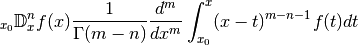
$\,_{x_0}{\mathbb{D}}^n_xf(x) \frac{1}{\Gamma(m-n)} \frac{d^m}{dx^m} \int_{x_0}^{x}(x-t)^{m-n-1}f(t)dt$

where $f$ is a given (presumably well-behaved) function, $x$ is the evaluation point, $n$ is the order, and $x_0$ is the reference point of integration ( $m$ is an arbitrary parameter selected automatically).

With $n = 1$ , this is just the standard derivative $f'(x)$ ; with $n = 2$ , the second derivative $f''(x)$ , etc. With $n = -1$ , it gives $\int_{x_0}^x f(t) dt$ , with $n = -2$ it gives $\int_{x_0}^x \left( \int_{x_0}^t f(u) du \right) dt$ , etc.

As $n$ is permitted to be any number, this operator generalizes iterated differentiation and iterated integration to a single operator with a continuous order parameter.

Examples

There is an exact formula for the fractional derivative of a monomial $x^p$ , which may be used as a reference. For example, the following gives a half-derivative (order 0.5):

>>> from mpmath import *
>>> mp.dps = 15; mp.pretty = True
>>> x = mpf(3); p = 2; n = 0.5
>>> differint(lambda t: t**p, x, n)
7.81764019044672
>>> gamma(p+1)/gamma(p-n+1) * x**(p-n)
7.81764019044672

Another useful test function is the exponential function, whose integration / differentiation formula easy generalizes to arbitrary order. Here we first compute a third derivative, and then a triply nested integral. (The reference point $x_0$ is set to $-\infty$ to avoid nonzero endpoint terms.):

>>> differint(lambda x: exp(pi*x), -1.5, 3)
0.278538406900792
>>> exp(pi*-1.5) * pi**3
0.278538406900792
>>> differint(lambda x: exp(pi*x), 3.5, -3, -inf)
1922.50563031149
>>> exp(pi*3.5) / pi**3
1922.50563031149

However, for noninteger $n$ , the differentiation formula for the exponential function must be modified to give the same result as the Riemann-Liouville differintegral:

>>> x = mpf(3.5)
>>> c = pi
>>> n = 1+2*j
>>> differint(lambda x: exp(c*x), x, n)
(-123295.005390743 + 140955.117867654j)
>>> x**(-n) * exp(c)**x * (x*c)**n * gammainc(-n, 0, x*c) / gamma(-n)
(-123295.005390743 + 140955.117867654j)

Differentiation¶

Numerical derivatives (`diff`, `diffs`)¶

Composition of derivatives (`diffs_prod`, `diffs_exp`)¶

Fractional derivatives / differintegration (`differint`)¶

Table Of Contents

Previous topic

Next topic

This Page

Navigation

Differentiation¶

Numerical derivatives (diff, diffs)¶

Composition of derivatives (diffs_prod, diffs_exp)¶

Fractional derivatives / differintegration (differint)¶

Table Of Contents

Previous topic

Next topic

This Page

Quick search

Navigation

Numerical derivatives (`diff`, `diffs`)¶

Composition of derivatives (`diffs_prod`, `diffs_exp`)¶

Fractional derivatives / differintegration (`differint`)¶