Sums, products, limits and extrapolation¶

The functions listed here permit approximation of infinite sums, products, and other sequence limits. Use mpmath.fsum() and mpmath.fprod() for summation and multiplication of finite sequences.

Summation¶

`nsum()`¶

mpmath.nsum(ctx, f, *intervals, **options)¶

Computes the sum

$S = \sum_{k=a}^b f(k)$

where $(a, b)$ = interval, and where $a = -\infty$ and/or $b = \infty$ are allowed, or more generally

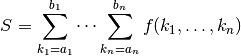
$S = \sum_{k_1=a_1}^{b_1} \cdots \sum_{k_n=a_n}^{b_n} f(k_1,\ldots,k_n)$

if multiple intervals are given.

Two examples of infinite series that can be summed by nsum(), where the first converges rapidly and the second converges slowly, are:

>>> from mpmath import *
>>> mp.dps = 15; mp.pretty = True
>>> nsum(lambda n: 1/fac(n), [0, inf])
2.71828182845905
>>> nsum(lambda n: 1/n**2, [1, inf])
1.64493406684823

When appropriate, nsum() applies convergence acceleration to accurately estimate the sums of slowly convergent series. If the series is finite, nsum() currently does not attempt to perform any extrapolation, and simply calls fsum().

Multidimensional infinite series are reduced to a single-dimensional series over expanding hypercubes; if both infinite and finite dimensions are present, the finite ranges are moved innermost. For more advanced control over the summation order, use nested calls to nsum(), or manually rewrite the sum as a single-dimensional series.

Options

tol: Desired maximum final error. Defaults roughly to the epsilon of the working precision.
method: Which summation algorithm to use (described below). Default: 'richardson+shanks'.
maxterms: Cancel after at most this many terms. Default: 10*dps.
steps: An iterable giving the number of terms to add between each extrapolation attempt. The default sequence is [10, 20, 30, 40, ...]. For example, if you know that approximately 100 terms will be required, efficiency might be improved by setting this to [100, 10]. Then the first extrapolation will be performed after 100 terms, the second after 110, etc.
verbose: Print details about progress.
ignore: If enabled, any term that raises ArithmeticError or ValueError (e.g. through division by zero) is replaced by a zero. This is convenient for lattice sums with a singular term near the origin.

Methods

Unfortunately, an algorithm that can efficiently sum any infinite series does not exist. nsum() implements several different algorithms that each work well in different cases. The method keyword argument selects a method.

The default method is 'r+s', i.e. both Richardson extrapolation and Shanks transformation is attempted. A slower method that handles more cases is 'r+s+e'. For very high precision summation, or if the summation needs to be fast (for example if multiple sums need to be evaluated), it is a good idea to investigate which one method works best and only use that.

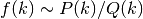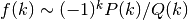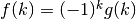
'richardson' / 'r':: Uses Richardson extrapolation. Provides useful extrapolation when $f(k) \sim P(k)/Q(k)$ or when $f(k) \sim (-1)^k P(k)/Q(k)$ for polynomials $P$ and $Q$ . See richardson() for additional information.
'shanks' / 's':: Uses Shanks transformation. Typically provides useful extrapolation when $f(k) \sim c^k$ or when successive terms alternate signs. Is able to sum some divergent series. See shanks() for additional information.
'levin' / 'l':: Uses the Levin transformation. It performs better than the Shanks transformation for logarithmic convergent or alternating divergent series. The 'levin_variant'-keyword selects the variant. Valid choices are “u”, “t”, “v” and “all” whereby “all” uses all three u,t and v simultanously (This is good for performance comparison in conjunction with “verbose=True”). Instead of the Levin transform one can also use the Sidi-S transform by selecting the method 'sidi'. See levin() for additional details.
'alternating' / 'a':: This is the convergence acceleration of alternating series developped by Cohen, Villegras and Zagier. See cohen_alt() for additional details.
'euler-maclaurin' / 'e':: Uses the Euler-Maclaurin summation formula to approximate the remainder sum by an integral. This requires high-order numerical derivatives and numerical integration. The advantage of this algorithm is that it works regardless of the decay rate of $f$ , as long as $f$ is sufficiently smooth. See sumem() for additional information.
'direct' / 'd':: Does not perform any extrapolation. This can be used (and should only be used for) rapidly convergent series. The summation automatically stops when the terms decrease below the target tolerance.

Basic examples

A finite sum:

>>> nsum(lambda k: 1/k, [1, 6])
2.45

Summation of a series going to negative infinity and a doubly infinite series:

>>> nsum(lambda k: 1/k**2, [-inf, -1])
1.64493406684823
>>> nsum(lambda k: 1/(1+k**2), [-inf, inf])
3.15334809493716

nsum() handles sums of complex numbers:

>>> nsum(lambda k: (0.5+0.25j)**k, [0, inf])
(1.6 + 0.8j)

The following sum converges very rapidly, so it is most efficient to sum it by disabling convergence acceleration:

>>> mp.dps = 1000
>>> a = nsum(lambda k: -(-1)**k * k**2 / fac(2*k), [1, inf],
...     method='direct')
>>> b = (cos(1)+sin(1))/4
>>> abs(a-b) < mpf('1e-998')
True

Examples with Richardson extrapolation

Richardson extrapolation works well for sums over rational functions, as well as their alternating counterparts:

>>> mp.dps = 50
>>> nsum(lambda k: 1 / k**3, [1, inf],
...     method='richardson')
1.2020569031595942853997381615114499907649862923405
>>> zeta(3)
1.2020569031595942853997381615114499907649862923405

>>> nsum(lambda n: (n + 3)/(n**3 + n**2), [1, inf],
...     method='richardson')
2.9348022005446793094172454999380755676568497036204
>>> pi**2/2-2
2.9348022005446793094172454999380755676568497036204

>>> nsum(lambda k: (-1)**k / k**3, [1, inf],
...     method='richardson')
-0.90154267736969571404980362113358749307373971925537
>>> -3*zeta(3)/4
-0.90154267736969571404980362113358749307373971925538

Examples with Shanks transformation

The Shanks transformation works well for geometric series and typically provides excellent acceleration for Taylor series near the border of their disk of convergence. Here we apply it to a series for $\log(2)$ , which can be seen as the Taylor series for $\log(1+x)$ with $x = 1$ :

>>> nsum(lambda k: -(-1)**k/k, [1, inf],
...     method='shanks')
0.69314718055994530941723212145817656807550013436025
>>> log(2)
0.69314718055994530941723212145817656807550013436025

Here we apply it to a slowly convergent geometric series:

>>> nsum(lambda k: mpf('0.995')**k, [0, inf],
...     method='shanks')
200.0

Finally, Shanks’ method works very well for alternating series where $f(k) = (-1)^k g(k)$ , and often does so regardless of the exact decay rate of $g(k)$ :

>>> mp.dps = 15
>>> nsum(lambda k: (-1)**(k+1) / k**1.5, [1, inf],
...     method='shanks')
0.765147024625408
>>> (2-sqrt(2))*zeta(1.5)/2
0.765147024625408

The following slowly convergent alternating series has no known closed-form value. Evaluating the sum a second time at higher precision indicates that the value is probably correct:

>>> nsum(lambda k: (-1)**k / log(k), [2, inf],
...     method='shanks')
0.924299897222939
>>> mp.dps = 30
>>> nsum(lambda k: (-1)**k / log(k), [2, inf],
...     method='shanks')
0.92429989722293885595957018136

Examples with Levin transformation

The following example calculates Euler’s constant as the constant term in the Laurent expansion of zeta(s) at s=1. This sum converges extremly slow because of the logarithmic convergence behaviour of the Dirichlet series for zeta.

>>> mp.dps = 30
>>> z = mp.mpf(10) ** (-10)
>>> a = mp.nsum(lambda n: n**(-(1+z)), [1, mp.inf], method = "levin") - 1 / z
>>> print(mp.chop(a - mp.euler, tol = 1e-10))
0.0

Now we sum the zeta function outside its range of convergence (attention: This does not work at the negative integers!):

>>> mp.dps = 15
>>> w = mp.nsum(lambda n: n ** (2 + 3j), [1, mp.inf], method = "levin", levin_variant = "v")
>>> print(mp.chop(w - mp.zeta(-2-3j)))
0.0

The next example resummates an asymptotic series expansion of an integral related to the exponential integral.

>>> mp.dps = 15
>>> z = mp.mpf(10)
>>> # exact = mp.quad(lambda x: mp.exp(-x)/(1+x/z),[0,mp.inf])
>>> exact = z * mp.exp(z) * mp.expint(1,z) # this is the symbolic expression for the integral
>>> w = mp.nsum(lambda n: (-1) ** n * mp.fac(n) * z ** (-n), [0, mp.inf], method = "sidi", levin_variant = "t")
>>> print(mp.chop(w - exact))
0.0

Following highly divergent asymptotic expansion needs some care. Firstly we need copious amount of working precision. Secondly the stepsize must not be chosen to large, otherwise nsum may miss the point where the Levin transform converges and reach the point where only numerical garbage is produced due to numerical cancellation.

>>> mp.dps = 15
>>> z = mp.mpf(2)
>>> # exact = mp.quad(lambda x: mp.exp( -x * x / 2 - z * x ** 4), [0,mp.inf]) * 2 / mp.sqrt(2 * mp.pi)
>>> exact = mp.exp(mp.one / (32 * z)) * mp.besselk(mp.one / 4, mp.one / (32 * z)) / (4 * mp.sqrt(z * mp.pi)) # this is the symbolic expression for the integral
>>> w = mp.nsum(lambda n: (-z)**n * mp.fac(4 * n) / (mp.fac(n) * mp.fac(2 * n) * (4 ** n)),
...   [0, mp.inf], method = "levin", levin_variant = "t", workprec = 8*mp.prec, steps = [2] + [1 for x in xrange(1000)])
>>> print(mp.chop(w - exact))
0.0

The hypergeoemtric function can also be summed outside its range of convergence:

>>> mp.dps = 15
>>> z = 2 + 1j
>>> exact = mp.hyp2f1(2 / mp.mpf(3), 4 / mp.mpf(3), 1 / mp.mpf(3), z)
>>> f = lambda n: mp.rf(2 / mp.mpf(3), n) * mp.rf(4 / mp.mpf(3), n) * z**n / (mp.rf(1 / mp.mpf(3), n) * mp.fac(n))
>>> v = mp.nsum(f, [0, mp.inf], method = "levin", steps = [10 for x in xrange(1000)])
>>> print(mp.chop(exact-v))
0.0

Examples with Cohen’s alternating series resummation

The next example sums the alternating zeta function:

>>> v = mp.nsum(lambda n: (-1)**(n-1) / n, [1, mp.inf], method = "a")
>>> print(mp.chop(v - mp.log(2)))
0.0

The derivate of the alternating zeta function outside its range of convergence:

>>> v = mp.nsum(lambda n: (-1)**n * mp.log(n) * n, [1, mp.inf], method = "a")
>>> print(mp.chop(v - mp.diff(lambda s: mp.altzeta(s), -1)))
0.0

Examples with Euler-Maclaurin summation

The sum in the following example has the wrong rate of convergence for either Richardson or Shanks to be effective.

>>> f = lambda k: log(k)/k**2.5
>>> mp.dps = 15
>>> nsum(f, [1, inf], method='euler-maclaurin')
0.38734195032621
>>> -diff(zeta, 2.5)
0.38734195032621

Increasing steps improves speed at higher precision:

>>> mp.dps = 50
>>> nsum(f, [1, inf], method='euler-maclaurin', steps=[250])
0.38734195032620997271199237593105101319948228874688
>>> -diff(zeta, 2.5)
0.38734195032620997271199237593105101319948228874688

Divergent series

The Shanks transformation is able to sum some divergent series. In particular, it is often able to sum Taylor series beyond their radius of convergence (this is due to a relation between the Shanks transformation and Pade approximations; see pade() for an alternative way to evaluate divergent Taylor series). Furthermore the Levin-transform examples above contain some divergent series resummation.

Here we apply it to $\log(1+x)$ far outside the region of convergence:

>>> mp.dps = 50
>>> nsum(lambda k: -(-9)**k/k, [1, inf],
...     method='shanks')
2.3025850929940456840179914546843642076011014886288
>>> log(10)
2.3025850929940456840179914546843642076011014886288

A particular type of divergent series that can be summed using the Shanks transformation is geometric series. The result is the same as using the closed-form formula for an infinite geometric series:

>>> mp.dps = 15
>>> for n in range(-8, 8):
...     if n == 1:
...         continue
...     print("%s %s %s" % (mpf(n), mpf(1)/(1-n),
...         nsum(lambda k: n**k, [0, inf], method='shanks')))
...
-8.0 0.111111111111111 0.111111111111111
-7.0 0.125 0.125
-6.0 0.142857142857143 0.142857142857143
-5.0 0.166666666666667 0.166666666666667
-4.0 0.2 0.2
-3.0 0.25 0.25
-2.0 0.333333333333333 0.333333333333333
-1.0 0.5 0.5
0.0 1.0 1.0
2.0 -1.0 -1.0
3.0 -0.5 -0.5
4.0 -0.333333333333333 -0.333333333333333
5.0 -0.25 -0.25
6.0 -0.2 -0.2
7.0 -0.166666666666667 -0.166666666666667

Multidimensional sums

Any combination of finite and infinite ranges is allowed for the summation indices:

>>> mp.dps = 15
>>> nsum(lambda x,y: x+y, [2,3], [4,5])
28.0
>>> nsum(lambda x,y: x/2**y, [1,3], [1,inf])
6.0
>>> nsum(lambda x,y: y/2**x, [1,inf], [1,3])
6.0
>>> nsum(lambda x,y,z: z/(2**x*2**y), [1,inf], [1,inf], [3,4])
7.0
>>> nsum(lambda x,y,z: y/(2**x*2**z), [1,inf], [3,4], [1,inf])
7.0
>>> nsum(lambda x,y,z: x/(2**z*2**y), [3,4], [1,inf], [1,inf])
7.0

Some nice examples of double series with analytic solutions or reductions to single-dimensional series (see [1]):

>>> nsum(lambda m, n: 1/2**(m*n), [1,inf], [1,inf])
1.60669515241529
>>> nsum(lambda n: 1/(2**n-1), [1,inf])
1.60669515241529

>>> nsum(lambda i,j: (-1)**(i+j)/(i**2+j**2), [1,inf], [1,inf])
0.278070510848213
>>> pi*(pi-3*ln2)/12
0.278070510848213

>>> nsum(lambda i,j: (-1)**(i+j)/(i+j)**2, [1,inf], [1,inf])
0.129319852864168
>>> altzeta(2) - altzeta(1)
0.129319852864168

>>> nsum(lambda i,j: (-1)**(i+j)/(i+j)**3, [1,inf], [1,inf])
0.0790756439455825
>>> altzeta(3) - altzeta(2)
0.0790756439455825

>>> nsum(lambda m,n: m**2*n/(3**m*(n*3**m+m*3**n)),
...     [1,inf], [1,inf])
0.28125
>>> mpf(9)/32
0.28125

>>> nsum(lambda i,j: fac(i-1)*fac(j-1)/fac(i+j),
...     [1,inf], [1,inf], workprec=400)
1.64493406684823
>>> zeta(2)
1.64493406684823

A hard example of a multidimensional sum is the Madelung constant in three dimensions (see [2]). The defining sum converges very slowly and only conditionally, so nsum() is lucky to obtain an accurate value through convergence acceleration. The second evaluation below uses a much more efficient, rapidly convergent 2D sum:

>>> nsum(lambda x,y,z: (-1)**(x+y+z)/(x*x+y*y+z*z)**0.5,
...     [-inf,inf], [-inf,inf], [-inf,inf], ignore=True)
-1.74756459463318
>>> nsum(lambda x,y: -12*pi*sech(0.5*pi * \
...     sqrt((2*x+1)**2+(2*y+1)**2))**2, [0,inf], [0,inf])
-1.74756459463318

Another example of a lattice sum in 2D:

>>> nsum(lambda x,y: (-1)**(x+y) / (x**2+y**2), [-inf,inf],
...     [-inf,inf], ignore=True)
-2.1775860903036
>>> -pi*ln2
-2.1775860903036

An example of an Eisenstein series:

>>> nsum(lambda m,n: (m+n*1j)**(-4), [-inf,inf], [-inf,inf],
...     ignore=True)
(3.1512120021539 + 0.0j)

References

`sumem()`¶

mpmath.sumem(ctx, f, interval, tol=None, reject=10, integral=None, adiffs=None, bdiffs=None, verbose=False, error=False, _fast_abort=False)¶

Uses the Euler-Maclaurin formula to compute an approximation accurate to within tol (which defaults to the present epsilon) of the sum

$S = \sum_{k=a}^b f(k)$

where $(a,b)$ are given by interval and $a$ or $b$ may be infinite. The approximation is

$S \sim \int_a^b f(x) \,dx + \frac{f(a)+f(b)}{2} + \sum_{k=1}^{\infty} \frac{B_{2k}}{(2k)!} \left(f^{(2k-1)}(b)-f^{(2k-1)}(a)\right).$

The last sum in the Euler-Maclaurin formula is not generally convergent (a notable exception is if $f$ is a polynomial, in which case Euler-Maclaurin actually gives an exact result).

The summation is stopped as soon as the quotient between two consecutive terms falls below reject. That is, by default (reject = 10), the summation is continued as long as each term adds at least one decimal.

Although not convergent, convergence to a given tolerance can often be “forced” if $b = \infty$ by summing up to $a+N$ and then applying the Euler-Maclaurin formula to the sum over the range $(a+N+1, \ldots, \infty)$ . This procedure is implemented by nsum().

By default numerical quadrature and differentiation is used. If the symbolic values of the integral and endpoint derivatives are known, it is more efficient to pass the value of the integral explicitly as integral and the derivatives explicitly as adiffs and bdiffs. The derivatives should be given as iterables that yield $f(a), f'(a), f''(a), \ldots$ (and the equivalent for $b$ ).

Examples

Summation of an infinite series, with automatic and symbolic integral and derivative values (the second should be much faster):

>>> from mpmath import *
>>> mp.dps = 50; mp.pretty = True
>>> sumem(lambda n: 1/n**2, [32, inf])
0.03174336652030209012658168043874142714132886413417
>>> I = mpf(1)/32
>>> D = adiffs=((-1)**n*fac(n+1)*32**(-2-n) for n in range(999))
>>> sumem(lambda n: 1/n**2, [32, inf], integral=I, adiffs=D)
0.03174336652030209012658168043874142714132886413417

An exact evaluation of a finite polynomial sum:

>>> sumem(lambda n: n**5-12*n**2+3*n, [-100000, 200000])
10500155000624963999742499550000.0
>>> print(sum(n**5-12*n**2+3*n for n in range(-100000, 200001)))
10500155000624963999742499550000

`sumap()`¶

mpmath.sumap(ctx, f, interval, integral=None, error=False)¶

Evaluates an infinite series of an analytic summand f using the Abel-Plana formula

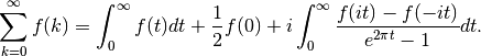
$\sum_{k=0}^{\infty} f(k) = \int_0^{\infty} f(t) dt + \frac{1}{2} f(0) + i \int_0^{\infty} \frac{f(it)-f(-it)}{e^{2\pi t}-1} dt.$

Unlike the Euler-Maclaurin formula (see sumem()), the Abel-Plana formula does not require derivatives. However, it only works when $|f(it)-f(-it)|$ does not increase too rapidly with $t$ .

Examples

The Abel-Plana formula is particularly useful when the summand decreases like a power of $k$ ; for example when the sum is a pure zeta function:

>>> from mpmath import *
>>> mp.dps = 25; mp.pretty = True
>>> sumap(lambda k: 1/k**2.5, [1,inf])
1.34148725725091717975677
>>> zeta(2.5)
1.34148725725091717975677
>>> sumap(lambda k: 1/(k+1j)**(2.5+2.5j), [1,inf])
(-3.385361068546473342286084 - 0.7432082105196321803869551j)
>>> zeta(2.5+2.5j, 1+1j)
(-3.385361068546473342286084 - 0.7432082105196321803869551j)

If the series is alternating, numerical quadrature along the real line is likely to give poor results, so it is better to evaluate the first term symbolically whenever possible:

>>> n=3; z=-0.75
>>> I = expint(n,-log(z))
>>> chop(sumap(lambda k: z**k / k**n, [1,inf], integral=I))
-0.6917036036904594510141448
>>> polylog(n,z)
-0.6917036036904594510141448

Products¶

`nprod()`¶

mpmath.nprod(ctx, f, interval, nsum=False, **kwargs)¶

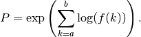
Computes the product

$P = \prod_{k=a}^b f(k)$

where $(a, b)$ = interval, and where $a = -\infty$ and/or $b = \infty$ are allowed.

By default, nprod() uses the same extrapolation methods as nsum(), except applied to the partial products rather than partial sums, and the same keyword options as for nsum() are supported. If nsum=True, the product is instead computed via nsum() as

$P = \exp\left( \sum_{k=a}^b \log(f(k)) \right).$

This is slower, but can sometimes yield better results. It is also required (and used automatically) when Euler-Maclaurin summation is requested.

Examples

A simple finite product:

>>> from mpmath import *
>>> mp.dps = 25; mp.pretty = True
>>> nprod(lambda k: k, [1, 4])
24.0

A large number of infinite products have known exact values, and can therefore be used as a reference. Most of the following examples are taken from MathWorld [1].

A few infinite products with simple values are:

>>> 2*nprod(lambda k: (4*k**2)/(4*k**2-1), [1, inf])
3.141592653589793238462643
>>> nprod(lambda k: (1+1/k)**2/(1+2/k), [1, inf])
2.0
>>> nprod(lambda k: (k**3-1)/(k**3+1), [2, inf])
0.6666666666666666666666667
>>> nprod(lambda k: (1-1/k**2), [2, inf])
0.5

Next, several more infinite products with more complicated values:

>>> nprod(lambda k: exp(1/k**2), [1, inf]); exp(pi**2/6)
5.180668317897115748416626
5.180668317897115748416626

>>> nprod(lambda k: (k**2-1)/(k**2+1), [2, inf]); pi*csch(pi)
0.2720290549821331629502366
0.2720290549821331629502366

>>> nprod(lambda k: (k**4-1)/(k**4+1), [2, inf])
0.8480540493529003921296502
>>> pi*sinh(pi)/(cosh(sqrt(2)*pi)-cos(sqrt(2)*pi))
0.8480540493529003921296502

>>> nprod(lambda k: (1+1/k+1/k**2)**2/(1+2/k+3/k**2), [1, inf])
1.848936182858244485224927
>>> 3*sqrt(2)*cosh(pi*sqrt(3)/2)**2*csch(pi*sqrt(2))/pi
1.848936182858244485224927

>>> nprod(lambda k: (1-1/k**4), [2, inf]); sinh(pi)/(4*pi)
0.9190194775937444301739244
0.9190194775937444301739244

>>> nprod(lambda k: (1-1/k**6), [2, inf])
0.9826842777421925183244759
>>> (1+cosh(pi*sqrt(3)))/(12*pi**2)
0.9826842777421925183244759

>>> nprod(lambda k: (1+1/k**2), [2, inf]); sinh(pi)/(2*pi)
1.838038955187488860347849
1.838038955187488860347849

>>> nprod(lambda n: (1+1/n)**n * exp(1/(2*n)-1), [1, inf])
1.447255926890365298959138
>>> exp(1+euler/2)/sqrt(2*pi)
1.447255926890365298959138

The following two products are equivalent and can be evaluated in terms of a Jacobi theta function. Pi can be replaced by any value (as long as convergence is preserved):

>>> nprod(lambda k: (1-pi**-k)/(1+pi**-k), [1, inf])
0.3838451207481672404778686
>>> nprod(lambda k: tanh(k*log(pi)/2), [1, inf])
0.3838451207481672404778686
>>> jtheta(4,0,1/pi)
0.3838451207481672404778686

This product does not have a known closed form value:

>>> nprod(lambda k: (1-1/2**k), [1, inf])
0.2887880950866024212788997

A product taken from $-\infty$ :

>>> nprod(lambda k: 1-k**(-3), [-inf,-2])
0.8093965973662901095786805
>>> cosh(pi*sqrt(3)/2)/(3*pi)
0.8093965973662901095786805

A doubly infinite product:

>>> nprod(lambda k: exp(1/(1+k**2)), [-inf, inf])
23.41432688231864337420035
>>> exp(pi/tanh(pi))
23.41432688231864337420035

A product requiring the use of Euler-Maclaurin summation to compute an accurate value:

>>> nprod(lambda k: (1-1/k**2.5), [2, inf], method='e')
0.696155111336231052898125

References

[Weisstein] http://mathworld.wolfram.com/InfiniteProduct.html

Limits (`limit`)¶

`limit()`¶

mpmath.limit(ctx, f, x, direction=1, exp=False, **kwargs)¶

Computes an estimate of the limit

$\lim_{t \to x} f(t)$

where $x$ may be finite or infinite.

For finite $x$ , limit() evaluates $f(x + d/n)$ for consecutive integer values of $n$ , where the approach direction $d$ may be specified using the direction keyword argument. For infinite $x$ , limit() evaluates values of $f(\mathrm{sign}(x) \cdot n)$ .

If the approach to the limit is not sufficiently fast to give an accurate estimate directly, limit() attempts to find the limit using Richardson extrapolation or the Shanks transformation. You can select between these methods using the method keyword (see documentation of nsum() for more information).

Options

The following options are available with essentially the same meaning as for nsum(): tol, method, maxterms, steps, verbose.

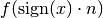
If the option exp=True is set, $f$ will be sampled at exponentially spaced points 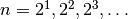$n = 2^1, 2^2, 2^3, \ldots$ instead of the linearly spaced points $n = 1, 2, 3, \ldots$ . This can sometimes improve the rate of convergence so that limit() may return a more accurate answer (and faster). However, do note that this can only be used if $f$ supports fast and accurate evaluation for arguments that are extremely close to the limit point (or if infinite, very large arguments).

Examples

A basic evaluation of a removable singularity:

>>> from mpmath import *
>>> mp.dps = 30; mp.pretty = True
>>> limit(lambda x: (x-sin(x))/x**3, 0)
0.166666666666666666666666666667

Computing the exponential function using its limit definition:

>>> limit(lambda n: (1+3/n)**n, inf)
20.0855369231876677409285296546
>>> exp(3)
20.0855369231876677409285296546

A limit for $\pi$ :

>>> f = lambda n: 2**(4*n+1)*fac(n)**4/(2*n+1)/fac(2*n)**2
>>> limit(f, inf)
3.14159265358979323846264338328

Calculating the coefficient in Stirling’s formula:

>>> limit(lambda n: fac(n) / (sqrt(n)*(n/e)**n), inf)
2.50662827463100050241576528481
>>> sqrt(2*pi)
2.50662827463100050241576528481

Evaluating Euler’s constant $\gamma$ using the limit representation

$\gamma = \lim_{n \rightarrow \infty } \left[ \left( \sum_{k=1}^n \frac{1}{k} \right) - \log(n) \right]$

(which converges notoriously slowly):

>>> f = lambda n: sum([mpf(1)/k for k in range(1,int(n)+1)]) - log(n)
>>> limit(f, inf)
0.577215664901532860606512090082
>>> +euler
0.577215664901532860606512090082

With default settings, the following limit converges too slowly to be evaluated accurately. Changing to exponential sampling however gives a perfect result:

>>> f = lambda x: sqrt(x**3+x**2)/(sqrt(x**3)+x)
>>> limit(f, inf)
0.992831158558330281129249686491
>>> limit(f, inf, exp=True)
1.0

Extrapolation¶

The following functions provide a direct interface to extrapolation algorithms. nsum() and limit() essentially work by calling the following functions with an increasing number of terms until the extrapolated limit is accurate enough.

The following functions may be useful to call directly if the precise number of terms needed to achieve a desired accuracy is known in advance, or if one wishes to study the convergence properties of the algorithms.

`richardson()`¶

mpmath.richardson(ctx, seq)¶

Given a list seq of the first $N$ elements of a slowly convergent infinite sequence, richardson() computes the $N$ -term Richardson extrapolate for the limit.

richardson() returns $(v, c)$ where $v$ is the estimated limit and $c$ is the magnitude of the largest weight used during the computation. The weight provides an estimate of the precision lost to cancellation. Due to cancellation effects, the sequence must be typically be computed at a much higher precision than the target accuracy of the extrapolation.

Applicability and issues

The $N$ -step Richardson extrapolation algorithm used by richardson() is described in [1].

Richardson extrapolation only works for a specific type of sequence, namely one converging like partial sums of $P(1)/Q(1) + P(2)/Q(2) + \ldots$ where $P$ and $Q$ are polynomials. When the sequence does not convergence at such a rate richardson() generally produces garbage.

Richardson extrapolation has the advantage of being fast: the $N$ -term extrapolate requires only $O(N)$ arithmetic operations, and usually produces an estimate that is accurate to $O(N)$ digits. Contrast with the Shanks transformation (see shanks()), which requires $O(N^2)$ operations.

richardson() is unable to produce an estimate for the approximation error. One way to estimate the error is to perform two extrapolations with slightly different $N$ and comparing the results.

Richardson extrapolation does not work for oscillating sequences. As a simple workaround, richardson() detects if the last three elements do not differ monotonically, and in that case applies extrapolation only to the even-index elements.

Example

Applying Richardson extrapolation to the Leibniz series for $\pi$ :

>>> from mpmath import *
>>> mp.dps = 30; mp.pretty = True
>>> S = [4*sum(mpf(-1)**n/(2*n+1) for n in range(m))
...     for m in range(1,30)]
>>> v, c = richardson(S[:10])
>>> v
3.2126984126984126984126984127
>>> nprint([v-pi, c])
[0.0711058, 2.0]

>>> v, c = richardson(S[:30])
>>> v
3.14159265468624052829954206226
>>> nprint([v-pi, c])
[1.09645e-9, 20833.3]

References

[BenderOrszag] pp. 375-376

`shanks()`¶

mpmath.shanks(ctx, seq, table=None, randomized=False)¶

Given a list seq of the first $N$ elements of a slowly convergent infinite sequence $(A_k)$ , shanks() computes the iterated Shanks transformation $S(A), S(S(A)), \ldots, S^{N/2}(A)$ . The Shanks transformation often provides strong convergence acceleration, especially if the sequence is oscillating.

The iterated Shanks transformation is computed using the Wynn epsilon algorithm (see [1]). shanks() returns the full epsilon table generated by Wynn’s algorithm, which can be read off as follows:

The table is a list of lists forming a lower triangular matrix, where higher row and column indices correspond to more accurate values.
The columns with even index hold dummy entries (required for the computation) and the columns with odd index hold the actual extrapolates.
The last element in the last row is typically the most accurate estimate of the limit.
The difference to the third last element in the last row provides an estimate of the approximation error.
The magnitude of the second last element provides an estimate of the numerical accuracy lost to cancellation.

For convenience, so the extrapolation is stopped at an odd index so that shanks(seq)[-1][-1] always gives an estimate of the limit.

Optionally, an existing table can be passed to shanks(). This can be used to efficiently extend a previous computation after new elements have been appended to the sequence. The table will then be updated in-place.

The Shanks transformation

The Shanks transformation is defined as follows (see [2]): given the input sequence $(A_0, A_1, \ldots)$ , the transformed sequence is given by

$S(A_k) = \frac{A_{k+1}A_{k-1}-A_k^2}{A_{k+1}+A_{k-1}-2 A_k}$

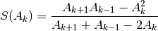
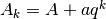The Shanks transformation gives the exact limit $A_{\infty}$ in a single step if $A_k = A + a q^k$ . Note in particular that it extrapolates the exact sum of a geometric series in a single step.

Applying the Shanks transformation once often improves convergence substantially for an arbitrary sequence, but the optimal effect is obtained by applying it iteratively: $S(S(A_k)), S(S(S(A_k))), \ldots$ .

Wynn’s epsilon algorithm provides an efficient way to generate the table of iterated Shanks transformations. It reduces the computation of each element to essentially a single division, at the cost of requiring dummy elements in the table. See [1] for details.

Precision issues

Due to cancellation effects, the sequence must be typically be computed at a much higher precision than the target accuracy of the extrapolation.

If the Shanks transformation converges to the exact limit (such as if the sequence is a geometric series), then a division by zero occurs. By default, shanks() handles this case by terminating the iteration and returning the table it has generated so far. With randomized=True, it will instead replace the zero by a pseudorandom number close to zero. (TODO: find a better solution to this problem.)

Examples

We illustrate by applying Shanks transformation to the Leibniz series for $\pi$ :

>>> from mpmath import *
>>> mp.dps = 50
>>> S = [4*sum(mpf(-1)**n/(2*n+1) for n in range(m))
...     for m in range(1,30)]
>>>
>>> T = shanks(S[:7])
>>> for row in T:
...     nprint(row)
...
[-0.75]
[1.25, 3.16667]
[-1.75, 3.13333, -28.75]
[2.25, 3.14524, 82.25, 3.14234]
[-2.75, 3.13968, -177.75, 3.14139, -969.937]
[3.25, 3.14271, 327.25, 3.14166, 3515.06, 3.14161]

The extrapolated accuracy is about 4 digits, and about 4 digits may have been lost due to cancellation:

>>> L = T[-1]
>>> nprint([abs(L[-1] - pi), abs(L[-1] - L[-3]), abs(L[-2])])
[2.22532e-5, 4.78309e-5, 3515.06]

Now we extend the computation:

>>> T = shanks(S[:25], T)
>>> L = T[-1]
>>> nprint([abs(L[-1] - pi), abs(L[-1] - L[-3]), abs(L[-2])])
[3.75527e-19, 1.48478e-19, 2.96014e+17]

The value for pi is now accurate to 18 digits. About 18 digits may also have been lost to cancellation.

Here is an example with a geometric series, where the convergence is immediate (the sum is exactly 1):

>>> mp.dps = 15
>>> for row in shanks([0.5, 0.75, 0.875, 0.9375, 0.96875]):
...     nprint(row)
[4.0]
[8.0, 1.0]

References

[GravesMorris]
[BenderOrszag] pp. 368-375

`levin()`¶

mpmath.levin(ctx, method='levin', variant='u')¶

This interface implements Levin’s (nonlinear) sequence transformation for convergence acceleration and summation of divergent series. It performs better than the Shanks/Wynn-epsilon algorithm for logarithmic convergent or alternating divergent series.

Let A be the series we want to sum:

$A = \sum_{k=0}^{\infty} a_k$

Attention: all $a_k$ must be non-zero!

Let $s_n$ be the partial sums of this series:

$s_n = \sum_{k=0}^n a_k.$

Methods

Calling levin returns an object with the following methods.

update(...) works with the list of individual terms $a_k$ of A, and update_step(...) works with the list of partial sums $s_k$ of A:

v, e = ...update([a_0, a_1,..., a_k])
v, e = ...update_psum([s_0, s_1,..., s_k])

step(...) works with the individual terms $a_k$ and step_psum(...) works with the partial sums $s_k$ :

v, e = ...step(a_k)
v, e = ...step_psum(s_k)

v is the current estimate for A, and e is an error estimate which is simply the difference between the current estimate and the last estimate. One should not mix update, update_psum, step and step_psum.

A word of caution

One can only hope for good results (i.e. convergence acceleration or resummation) if the $s_n$ have some well defind asymptotic behavior for large $n$ and are not erratic or random. Furthermore one usually needs very high working precision because of the numerical cancellation. If the working precision is insufficient, levin may produce silently numerical garbage. Furthermore even if the Levin-transformation converges, in the general case there is no proof that the result is mathematically sound. Only for very special classes of problems one can prove that the Levin-transformation converges to the expected result (for example Stieltjes-type integrals). Furthermore the Levin-transform is quite expensive (i.e. slow) in comparison to Shanks/Wynn-epsilon, Richardson & co. In summary one can say that the Levin-transformation is powerful but unreliable and that it may need a copious amount of working precision.

The Levin transform has several variants differing in the choice of weights. Some variants are better suited for the possible flavours of convergence behaviour of A than other variants:

convergence behaviour   levin-u   levin-t   levin-v   shanks/wynn-epsilon

logarithmic               +         -         +           -
linear                    +         +         +           +
alternating divergent     +         +         +           +

  "+" means the variant is suitable,"-" means the variant is not suitable;
  for comparison the Shanks/Wynn-epsilon transform is listed, too.

The variant is controlled though the variant keyword (i.e. variant="u", variant="t" or variant="v"). Overall “u” is probably the best choice.

Finally it is possible to use the Sidi-S transform instead of the Levin transform by using the keyword method='sidi'. The Sidi-S transform works better than the Levin transformation for some divergent series (see the examples).

Parameters:

method      "levin" or "sidi" chooses either the Levin or the Sidi-S transformation
variant     "u","t" or "v" chooses the weight variant.

The Levin transform is also accessible through the nsum interface. method="l" or method="levin" select the normal Levin transform while method="sidi" selects the Sidi-S transform. The variant is in both cases selected through the levin_variant keyword. The stepsize in nsum() must not be chosen too large, otherwise it will miss the point where the Levin transform converges resulting in numerical overflow/garbage. For highly divergent series a copious amount of working precision must be chosen.

Examples

First we sum the zeta function:

>>> from mpmath import mp
>>> mp.prec = 53
>>> eps = mp.mpf(mp.eps)
>>> with mp.extraprec(2 * mp.prec): # levin needs a high working precision
...     L = mp.levin(method = "levin", variant = "u")
...     S, s, n = [], 0, 1
...     while 1:
...         s += mp.one / (n * n)
...         n += 1
...         S.append(s)
...         v, e = L.update_psum(S)
...         if e < eps:
...             break
...         if n > 1000: raise RuntimeError("iteration limit exceeded")
>>> print(mp.chop(v - mp.pi ** 2 / 6))
0.0
>>> w = mp.nsum(lambda n: 1 / (n*n), [1, mp.inf], method = "levin", levin_variant = "u")
>>> print(mp.chop(v - w))
0.0

Now we sum the zeta function outside its range of convergence (attention: This does not work at the negative integers!):

>>> eps = mp.mpf(mp.eps)
>>> with mp.extraprec(2 * mp.prec): # levin needs a high working precision
...     L = mp.levin(method = "levin", variant = "v")
...     A, n = [], 1
...     while 1:
...         s = mp.mpf(n) ** (2 + 3j)
...         n += 1
...         A.append(s)
...         v, e = L.update(A)
...         if e < eps:
...             break
...         if n > 1000: raise RuntimeError("iteration limit exceeded")
>>> print(mp.chop(v - mp.zeta(-2-3j)))
0.0
>>> w = mp.nsum(lambda n: n ** (2 + 3j), [1, mp.inf], method = "levin", levin_variant = "v")
>>> print(mp.chop(v - w))
0.0

Now we sum the divergent asymptotic expansion of an integral related to the exponential integral (see also [2] p.373). The Sidi-S transform works best here:

>>> z = mp.mpf(10)
>>> exact = mp.quad(lambda x: mp.exp(-x)/(1+x/z),[0,mp.inf])
>>> # exact = z * mp.exp(z) * mp.expint(1,z) # this is the symbolic expression for the integral
>>> eps = mp.mpf(mp.eps)
>>> with mp.extraprec(2 * mp.prec): # high working precisions are mandatory for divergent resummation
...     L = mp.levin(method = "sidi", variant = "t")
...     n = 0
...     while 1:
...         s = (-1)**n * mp.fac(n) * z ** (-n)
...         v, e = L.step(s)
...         n += 1
...         if e < eps:
...             break
...         if n > 1000: raise RuntimeError("iteration limit exceeded")
>>> print(mp.chop(v - exact))
0.0
>>> w = mp.nsum(lambda n: (-1) ** n * mp.fac(n) * z ** (-n), [0, mp.inf], method = "sidi", levin_variant = "t")
>>> print(mp.chop(v - w))
0.0

Another highly divergent integral is also summable:

>>> z = mp.mpf(2)
>>> eps = mp.mpf(mp.eps)
>>> exact = mp.quad(lambda x: mp.exp( -x * x / 2 - z * x ** 4), [0,mp.inf]) * 2 / mp.sqrt(2 * mp.pi)
>>> # exact = mp.exp(mp.one / (32 * z)) * mp.besselk(mp.one / 4, mp.one / (32 * z)) / (4 * mp.sqrt(z * mp.pi)) # this is the symbolic expression for the integral
>>> with mp.extraprec(7 * mp.prec):  # we need copious amount of precision to sum this highly divergent series
...     L = mp.levin(method = "levin", variant = "t")
...     n, s = 0, 0
...     while 1:
...         s += (-z)**n * mp.fac(4 * n) / (mp.fac(n) * mp.fac(2 * n) * (4 ** n))
...         n += 1
...         v, e = L.step_psum(s)
...         if e < eps:
...             break
...         if n > 1000: raise RuntimeError("iteration limit exceeded")
>>> print(mp.chop(v - exact))
0.0
>>> w = mp.nsum(lambda n: (-z)**n * mp.fac(4 * n) / (mp.fac(n) * mp.fac(2 * n) * (4 ** n)),
...   [0, mp.inf], method = "levin", levin_variant = "t", workprec = 8*mp.prec, steps = [2] + [1 for x in xrange(1000)])
>>> print(mp.chop(v - w))
0.0

These examples run with 15-20 decimal digits precision. For higher precision the working precision must be raised.

Examples for nsum

Here we calculate Euler’s constant as the constant term in the Laurent expansion of $\zeta(s)$ at $s=1$ . This sum converges extremly slowly because of the logarithmic convergence behaviour of the Dirichlet series for zeta:

>>> mp.dps = 30
>>> z = mp.mpf(10) ** (-10)
>>> a = mp.nsum(lambda n: n**(-(1+z)), [1, mp.inf], method = "l") - 1 / z
>>> print(mp.chop(a - mp.euler, tol = 1e-10))
0.0

The Sidi-S transform performs excellently for the alternating series of $\log(2)$ :

>>> a = mp.nsum(lambda n: (-1)**(n-1) / n, [1, mp.inf], method = "sidi")
>>> print(mp.chop(a - mp.log(2)))
0.0

Hypergeometric series can also be summed outside their range of convergence. The stepsize in nsum() must not be chosen too large, otherwise it will miss the point where the Levin transform converges resulting in numerical overflow/garbage:

>>> z = 2 + 1j
>>> exact = mp.hyp2f1(2 / mp.mpf(3), 4 / mp.mpf(3), 1 / mp.mpf(3), z)
>>> f = lambda n: mp.rf(2 / mp.mpf(3), n) * mp.rf(4 / mp.mpf(3), n) * z**n / (mp.rf(1 / mp.mpf(3), n) * mp.fac(n))
>>> v = mp.nsum(f, [0, mp.inf], method = "levin", steps = [10 for x in xrange(1000)])
>>> print(mp.chop(exact-v))
0.0

References:

[1] E.J. Weniger - “Nonlinear Sequence Transformations for the Acceleration of

Convergence and the Summation of Divergent Series” arXiv:math/0306302

[2] A. Sidi - “Pratical Extrapolation Methods”

[3] H.H.H. Homeier - “Scalar Levin-Type Sequence Transformations” arXiv:math/0005209

`cohen_alt()`¶

mpmath.cohen_alt(ctx)¶

This interface implements the convergence acceleration of alternating series as described in H. Cohen, F.R. Villegas, D. Zagier - “Convergence Acceleration of Alternating Series”. This series transformation works only well if the individual terms of the series have an alternating sign. It belongs to the class of linear series transformations (in contrast to the Shanks/Wynn-epsilon or Levin transform). This series transformation is also able to sum some types of divergent series. See the paper under which conditions this resummation is mathematical sound.

Let A be the series we want to sum:

$A = \sum_{k=0}^{\infty} a_k$

Let $s_n$ be the partial sums of this series:

$s_n = \sum_{k=0}^n a_k.$

Interface

Calling cohen_alt returns an object with the following methods.

Then update(...) works with the list of individual terms $a_k$ and update_psum(...) works with the list of partial sums $s_k$ :

v, e = ...update([a_0, a_1,..., a_k])
v, e = ...update_psum([s_0, s_1,..., s_k])

v is the current estimate for A, and e is an error estimate which is simply the difference between the current estimate and the last estimate.

Examples

Here we compute the alternating zeta function using update_psum:

>>> from mpmath import mp
>>> AC = mp.cohen_alt()
>>> S, s, n = [], 0, 1
>>> while 1:
...     s += -((-1) ** n) * mp.one / (n * n)
...     n += 1
...     S.append(s)
...     v, e = AC.update_psum(S)
...     if e < mp.eps:
...         break
...     if n > 1000: raise RuntimeError("iteration limit exceeded")
>>> print(mp.chop(v - mp.pi ** 2 / 12))
0.0

Here we compute the product $\prod_{n=1}^{\infty} \Gamma(1+1/(2n-1)) / \Gamma(1+1/(2n))$ :

>>> A = []
>>> AC = mp.cohen_alt()
>>> n = 1
>>> while 1:
...     A.append( mp.loggamma(1 + mp.one / (2 * n - 1)))
...     A.append(-mp.loggamma(1 + mp.one / (2 * n)))
...     n += 1
...     v, e = AC.update(A)
...     if e < mp.eps:
...         break
...     if n > 1000: raise RuntimeError("iteration limit exceeded")
>>> v = mp.exp(v)
>>> print(mp.chop(v - 1.06215090557106, tol = 1e-12))
0.0

cohen_alt is also accessible through the nsum() interface:

>>> v = mp.nsum(lambda n: (-1)**(n-1) / n, [1, mp.inf], method = "a")
>>> print(mp.chop(v - mp.log(2)))
0.0
>>> v = mp.nsum(lambda n: (-1)**n / (2 * n + 1), [0, mp.inf], method = "a")
>>> print(mp.chop(v - mp.pi / 4))
0.0
>>> v = mp.nsum(lambda n: (-1)**n * mp.log(n) * n, [1, mp.inf], method = "a")
>>> print(mp.chop(v - mp.diff(lambda s: mp.altzeta(s), -1)))
0.0

Sums, products, limits and extrapolation¶

Summation¶

`nsum()`¶

`sumem()`¶

`sumap()`¶

Products¶

`nprod()`¶

Limits (`limit`)¶

`limit()`¶

Extrapolation¶

`richardson()`¶

`shanks()`¶

`levin()`¶

`cohen_alt()`¶

Table Of Contents

Previous topic

Next topic

This Page

Navigation

Sums, products, limits and extrapolation¶

Summation¶

nsum()¶

sumem()¶

sumap()¶

Products¶

nprod()¶

Limits (limit)¶

limit()¶

Extrapolation¶

richardson()¶

shanks()¶

levin()¶

cohen_alt()¶

Table Of Contents

Previous topic

Next topic

This Page

Quick search

Navigation

`nsum()`¶

`sumem()`¶

`sumap()`¶

`nprod()`¶

Limits (`limit`)¶

`limit()`¶

`richardson()`¶

`shanks()`¶

`levin()`¶

`cohen_alt()`¶