Trigonometric functions¶

Except where otherwise noted, the trigonometric functions take a radian angle as input and the inverse trigonometric functions return radian angles.

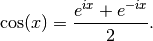
The ordinary trigonometric functions are single-valued functions defined everywhere in the complex plane (except at the poles of tan, sec, csc, and cot). They are defined generally via the exponential function, e.g.

$\cos(x) = \frac{e^{ix} + e^{-ix}}{2}.$

The inverse trigonometric functions are multivalued, thus requiring branch cuts, and are generally real-valued only on a part of the real line. Definitions and branch cuts are given in the documentation of each function. The branch cut conventions used by mpmath are essentially the same as those found in most standard mathematical software, such as Mathematica and Python’s own cmath libary (as of Python 2.6; earlier Python versions implement some functions erroneously).

Degree-radian conversion¶

`degrees()`¶

mpmath.degrees(x)¶

Converts the radian angle $x$ to a degree angle:

>>> from mpmath import *
>>> mp.dps = 15; mp.pretty = True
>>> degrees(pi/3)
60.0

`radians()`¶

mpmath.radians(x)¶

Converts the degree angle $x$ to radians:

>>> from mpmath import *
>>> mp.dps = 15; mp.pretty = True
>>> radians(60)
1.0471975511966

Trigonometric functions¶

`cos()`¶

mpmath.cos(x, **kwargs)¶

Computes the cosine of $x$ , $\cos(x)$ .

>>> from mpmath import *
>>> mp.dps = 25; mp.pretty = True
>>> cos(pi/3)
0.5
>>> cos(100000001)
-0.9802850113244713353133243
>>> cos(2+3j)
(-4.189625690968807230132555 - 9.109227893755336597979197j)
>>> cos(inf)
nan
>>> nprint(chop(taylor(cos, 0, 6)))
[1.0, 0.0, -0.5, 0.0, 0.0416667, 0.0, -0.00138889]

Intervals are supported via mpmath.iv.cos():

>>> iv.dps = 25; iv.pretty = True
>>> iv.cos([0,1])
[0.540302305868139717400936602301, 1.0]
>>> iv.cos([0,2])
[-0.41614683654714238699756823214, 1.0]

`sin()`¶

mpmath.sin(x, **kwargs)¶

Computes the sine of $x$ , $\sin(x)$ .

>>> from mpmath import *
>>> mp.dps = 25; mp.pretty = True
>>> sin(pi/3)
0.8660254037844386467637232
>>> sin(100000001)
0.1975887055794968911438743
>>> sin(2+3j)
(9.1544991469114295734673 - 4.168906959966564350754813j)
>>> sin(inf)
nan
>>> nprint(chop(taylor(sin, 0, 6)))
[0.0, 1.0, 0.0, -0.166667, 0.0, 0.00833333, 0.0]

Intervals are supported via mpmath.iv.sin():

>>> iv.dps = 25; iv.pretty = True
>>> iv.sin([0,1])
[0.0, 0.841470984807896506652502331201]
>>> iv.sin([0,2])
[0.0, 1.0]

`tan()`¶

mpmath.tan(x, **kwargs)¶

Computes the tangent of $x$ , $\tan(x) = \frac{\sin(x)}{\cos(x)}$ . The tangent function is singular at $x = (n+1/2)\pi$ , but tan(x) always returns a finite result since $(n+1/2)\pi$ cannot be represented exactly using floating-point arithmetic.

>>> from mpmath import *
>>> mp.dps = 25; mp.pretty = True
>>> tan(pi/3)
1.732050807568877293527446
>>> tan(100000001)
-0.2015625081449864533091058
>>> tan(2+3j)
(-0.003764025641504248292751221 + 1.003238627353609801446359j)
>>> tan(inf)
nan
>>> nprint(chop(taylor(tan, 0, 6)))
[0.0, 1.0, 0.0, 0.333333, 0.0, 0.133333, 0.0]

Intervals are supported via mpmath.iv.tan():

>>> iv.dps = 25; iv.pretty = True
>>> iv.tan([0,1])
[0.0, 1.55740772465490223050697482944]
>>> iv.tan([0,2])  # Interval includes a singularity
[-inf, +inf]

`sec()`¶

mpmath.sec(x)¶

Computes the secant of $x$ , $\mathrm{sec}(x) = \frac{1}{\cos(x)}$ . The secant function is singular at $x = (n+1/2)\pi$ , but sec(x) always returns a finite result since $(n+1/2)\pi$ cannot be represented exactly using floating-point arithmetic.

>>> from mpmath import *
>>> mp.dps = 25; mp.pretty = True
>>> sec(pi/3)
2.0
>>> sec(10000001)
-1.184723164360392819100265
>>> sec(2+3j)
(-0.04167496441114427004834991 + 0.0906111371962375965296612j)
>>> sec(inf)
nan
>>> nprint(chop(taylor(sec, 0, 6)))
[1.0, 0.0, 0.5, 0.0, 0.208333, 0.0, 0.0847222]

Intervals are supported via mpmath.iv.sec():

>>> iv.dps = 25; iv.pretty = True
>>> iv.sec([0,1])
[1.0, 1.85081571768092561791175326276]
>>> iv.sec([0,2])  # Interval includes a singularity
[-inf, +inf]

`csc()`¶

mpmath.csc(x)¶

Computes the cosecant of $x$ , $\mathrm{csc}(x) = \frac{1}{\sin(x)}$ . This cosecant function is singular at $x = n \pi$ , but with the exception of the point $x = 0$ , csc(x) returns a finite result since $n \pi$ cannot be represented exactly using floating-point arithmetic.

>>> from mpmath import *
>>> mp.dps = 25; mp.pretty = True
>>> csc(pi/3)
1.154700538379251529018298
>>> csc(10000001)
-1.864910497503629858938891
>>> csc(2+3j)
(0.09047320975320743980579048 + 0.04120098628857412646300981j)
>>> csc(inf)
nan

Intervals are supported via mpmath.iv.csc():

>>> iv.dps = 25; iv.pretty = True
>>> iv.csc([0,1])  # Interval includes a singularity
[1.18839510577812121626159943988, +inf]
>>> iv.csc([0,2])
[1.0, +inf]

`cot()`¶

mpmath.cot(x)¶

Computes the cotangent of $x$ , $\mathrm{cot}(x) = \frac{1}{\tan(x)} = \frac{\cos(x)}{\sin(x)}$ . This cotangent function is singular at $x = n \pi$ , but with the exception of the point $x = 0$ , cot(x) returns a finite result since $n \pi$ cannot be represented exactly using floating-point arithmetic.

>>> from mpmath import *
>>> mp.dps = 25; mp.pretty = True
>>> cot(pi/3)
0.5773502691896257645091488
>>> cot(10000001)
1.574131876209625656003562
>>> cot(2+3j)
(-0.003739710376336956660117409 - 0.9967577965693583104609688j)
>>> cot(inf)
nan

Intervals are supported via mpmath.iv.cot():

>>> iv.dps = 25; iv.pretty = True
>>> iv.cot([0,1])  # Interval includes a singularity
[0.642092615934330703006419974862, +inf]
>>> iv.cot([1,2])
[-inf, +inf]

Trigonometric functions with modified argument¶

`cospi()`¶

mpmath.cospi(x, **kwargs)¶

Computes $\cos(\pi x)$ , more accurately than the expression cos(pi*x):

>>> from mpmath import *
>>> mp.dps = 15; mp.pretty = True
>>> cospi(10**10), cos(pi*(10**10))
(1.0, 0.999999999997493)
>>> cospi(10**10+0.5), cos(pi*(10**10+0.5))
(0.0, 1.59960492420134e-6)

`sinpi()`¶

mpmath.sinpi(x, **kwargs)¶

Computes $\sin(\pi x)$ , more accurately than the expression sin(pi*x):

>>> from mpmath import *
>>> mp.dps = 15; mp.pretty = True
>>> sinpi(10**10), sin(pi*(10**10))
(0.0, -2.23936276195592e-6)
>>> sinpi(10**10+0.5), sin(pi*(10**10+0.5))
(1.0, 0.999999999998721)

Inverse trigonometric functions¶

`acos()`¶

mpmath.acos(x, **kwargs)¶

Computes the inverse cosine or arccosine of $x$ , $\cos^{-1}(x)$ . Since $-1 \le \cos(x) \le 1$ for real $x$ , the inverse cosine is real-valued only for $-1 \le x \le 1$ . On this interval, acos() is defined to be a monotonically decreasing function assuming values between $+\pi$ and $0$ .

Basic values are:

>>> from mpmath import *
>>> mp.dps = 25; mp.pretty = True
>>> acos(-1)
3.141592653589793238462643
>>> acos(0)
1.570796326794896619231322
>>> acos(1)
0.0
>>> nprint(chop(taylor(acos, 0, 6)))
[1.5708, -1.0, 0.0, -0.166667, 0.0, -0.075, 0.0]

acos() is defined so as to be a proper inverse function of $\cos(\theta)$ for $0 \le \theta < \pi$ . We have $\cos(\cos^{-1}(x)) = x$ for all $x$ , but $\cos^{-1}(\cos(x)) = x$ only for $0 \le \Re[x] < \pi$ :

>>> for x in [1, 10, -1, 2+3j, 10+3j]:
...     print("%s %s" % (cos(acos(x)), acos(cos(x))))
...
1.0 1.0
(10.0 + 0.0j) 2.566370614359172953850574
-1.0 1.0
(2.0 + 3.0j) (2.0 + 3.0j)
(10.0 + 3.0j) (2.566370614359172953850574 - 3.0j)

The inverse cosine has two branch points: $x = \pm 1$ . acos() places the branch cuts along the line segments $(-\infty, -1)$ and $(+1, +\infty)$ . In general,

$\cos^{-1}(x) = \frac{\pi}{2} + i \log\left(ix + \sqrt{1-x^2} \right)$

where the principal-branch log and square root are implied.

`asin()`¶

mpmath.asin(x, **kwargs)¶

Computes the inverse sine or arcsine of $x$ , $\sin^{-1}(x)$ . Since $-1 \le \sin(x) \le 1$ for real $x$ , the inverse sine is real-valued only for $-1 \le x \le 1$ . On this interval, it is defined to be a monotonically increasing function assuming values between $-\pi/2$ and $\pi/2$ .

Basic values are:

>>> from mpmath import *
>>> mp.dps = 25; mp.pretty = True
>>> asin(-1)
-1.570796326794896619231322
>>> asin(0)
0.0
>>> asin(1)
1.570796326794896619231322
>>> nprint(chop(taylor(asin, 0, 6)))
[0.0, 1.0, 0.0, 0.166667, 0.0, 0.075, 0.0]

asin() is defined so as to be a proper inverse function of $\sin(\theta)$ for $-\pi/2 < \theta < \pi/2$ . We have $\sin(\sin^{-1}(x)) = x$ for all $x$ , but $\sin^{-1}(\sin(x)) = x$ only for $-\pi/2 < \Re[x] < \pi/2$ :

>>> for x in [1, 10, -1, 1+3j, -2+3j]:
...     print("%s %s" % (chop(sin(asin(x))), asin(sin(x))))
...
1.0 1.0
10.0 -0.5752220392306202846120698
-1.0 -1.0
(1.0 + 3.0j) (1.0 + 3.0j)
(-2.0 + 3.0j) (-1.141592653589793238462643 - 3.0j)

The inverse sine has two branch points: $x = \pm 1$ . asin() places the branch cuts along the line segments $(-\infty, -1)$ and $(+1, +\infty)$ . In general,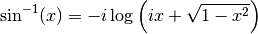

$\sin^{-1}(x) = -i \log\left(ix + \sqrt{1-x^2} \right)$

where the principal-branch log and square root are implied.

`atan()`¶

mpmath.atan(x, **kwargs)¶

Computes the inverse tangent or arctangent of $x$ , $\tan^{-1}(x)$ . This is a real-valued function for all real $x$ , with range $(-\pi/2, \pi/2)$ .

Basic values are:

>>> from mpmath import *
>>> mp.dps = 25; mp.pretty = True
>>> atan(-inf)
-1.570796326794896619231322
>>> atan(-1)
-0.7853981633974483096156609
>>> atan(0)
0.0
>>> atan(1)
0.7853981633974483096156609
>>> atan(inf)
1.570796326794896619231322
>>> nprint(chop(taylor(atan, 0, 6)))
[0.0, 1.0, 0.0, -0.333333, 0.0, 0.2, 0.0]

The inverse tangent is often used to compute angles. However, the atan2 function is often better for this as it preserves sign (see atan2()).

atan() is defined so as to be a proper inverse function of $\tan(\theta)$ for $-\pi/2 < \theta < \pi/2$ . We have $\tan(\tan^{-1}(x)) = x$ for all $x$ , but $\tan^{-1}(\tan(x)) = x$ only for $-\pi/2 < \Re[x] < \pi/2$ :

>>> mp.dps = 25
>>> for x in [1, 10, -1, 1+3j, -2+3j]:
...     print("%s %s" % (tan(atan(x)), atan(tan(x))))
...
1.0 1.0
10.0 0.5752220392306202846120698
-1.0 -1.0
(1.0 + 3.0j) (1.000000000000000000000001 + 3.0j)
(-2.0 + 3.0j) (1.141592653589793238462644 + 3.0j)

The inverse tangent has two branch points: $x = \pm i$ . atan() places the branch cuts along the line segments $(-i \infty, -i)$ and $(+i, +i \infty)$ . In general,

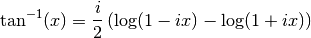
$\tan^{-1}(x) = \frac{i}{2}\left(\log(1-ix)-\log(1+ix)\right)$

where the principal-branch log is implied.

`atan2()`¶

mpmath.atan2(y, x)¶

Computes the two-argument arctangent, $\mathrm{atan2}(y, x)$ , giving the signed angle between the positive $x$ -axis and the point $(x, y)$ in the 2D plane. This function is defined for real $x$ and $y$ only.

The two-argument arctangent essentially computes $\mathrm{atan}(y/x)$ , but accounts for the signs of both $x$ and $y$ to give the angle for the correct quadrant. The following examples illustrate the difference:

>>> from mpmath import *
>>> mp.dps = 15; mp.pretty = True
>>> atan2(1,1), atan(1/1.)
(0.785398163397448, 0.785398163397448)
>>> atan2(1,-1), atan(1/-1.)
(2.35619449019234, -0.785398163397448)
>>> atan2(-1,1), atan(-1/1.)
(-0.785398163397448, -0.785398163397448)
>>> atan2(-1,-1), atan(-1/-1.)
(-2.35619449019234, 0.785398163397448)

The angle convention is the same as that used for the complex argument; see arg().

`asec()`¶

mpmath.asec(x)¶: Computes the inverse secant of $x$ , $\mathrm{sec}^{-1}(x) = \cos^{-1}(1/x)$ .

`acsc()`¶

mpmath.acsc(x)¶: Computes the inverse cosecant of $x$ , $\mathrm{csc}^{-1}(x) = \sin^{-1}(1/x)$ .

`acot()`¶

mpmath.acot(x)¶: Computes the inverse cotangent of $x$ , $\mathrm{cot}^{-1}(x) = \tan^{-1}(1/x)$ .

Sinc function¶

`sinc()`¶

mpmath.sinc(x)¶

sinc(x) computes the unnormalized sinc function, defined as

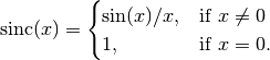
$\mathrm{sinc}(x) = \begin{cases} \sin(x)/x, & \mbox{if } x \ne 0 \\ 1, & \mbox{if } x = 0. \end{cases}$

See sincpi() for the normalized sinc function.

Simple values and limits include:

>>> from mpmath import *
>>> mp.dps = 15; mp.pretty = True
>>> sinc(0)
1.0
>>> sinc(1)
0.841470984807897
>>> sinc(inf)
0.0

The integral of the sinc function is the sine integral Si:

>>> quad(sinc, [0, 1])
0.946083070367183
>>> si(1)
0.946083070367183

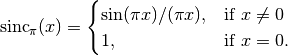
`sincpi()`¶

mpmath.sincpi(x)¶

sincpi(x) computes the normalized sinc function, defined as

$\mathrm{sinc}_{\pi}(x) = \begin{cases} \sin(\pi x)/(\pi x), & \mbox{if } x \ne 0 \\ 1, & \mbox{if } x = 0. \end{cases}$

Equivalently, we have $\mathrm{sinc}_{\pi}(x) = \mathrm{sinc}(\pi x)$ .

The normalization entails that the function integrates to unity over the entire real line:

>>> from mpmath import *
>>> mp.dps = 15; mp.pretty = True
>>> quadosc(sincpi, [-inf, inf], period=2.0)
1.0

Like, sinpi(), sincpi() is evaluated accurately at its roots:

>>> sincpi(10)
0.0

Trigonometric functions¶

Degree-radian conversion¶

`degrees()`¶

`radians()`¶

Trigonometric functions¶

`cos()`¶

`sin()`¶

`tan()`¶

`sec()`¶

`csc()`¶

`cot()`¶

Trigonometric functions with modified argument¶

`cospi()`¶

`sinpi()`¶

Inverse trigonometric functions¶

`acos()`¶

`asin()`¶

`atan()`¶

`atan2()`¶

`asec()`¶

`acsc()`¶

`acot()`¶

Sinc function¶

`sinc()`¶

`sincpi()`¶

Table Of Contents

Previous topic

Next topic

This Page

Navigation

Trigonometric functions¶

Degree-radian conversion¶

degrees()¶

radians()¶

Trigonometric functions¶

cos()¶

sin()¶

tan()¶

sec()¶

csc()¶

cot()¶

Trigonometric functions with modified argument¶

cospi()¶

sinpi()¶

Inverse trigonometric functions¶

acos()¶

asin()¶

atan()¶

atan2()¶

asec()¶

acsc()¶

acot()¶

Sinc function¶

sinc()¶

sincpi()¶

Table Of Contents

Previous topic

Next topic

This Page

Quick search

Navigation

`degrees()`¶

`radians()`¶

`cos()`¶

`sin()`¶

`tan()`¶

`sec()`¶

`csc()`¶

`cot()`¶

`cospi()`¶

`sinpi()`¶

`acos()`¶

`asin()`¶

`atan()`¶

`atan2()`¶

`asec()`¶

`acsc()`¶

`acot()`¶

`sinc()`¶

`sincpi()`¶