Powers and logarithms¶

Nth roots¶

`sqrt()`¶

mpmath.sqrt(x, **kwargs)¶

sqrt(x) gives the principal square root of $x$ , $\sqrt x$ . For positive real numbers, the principal root is simply the positive square root. For arbitrary complex numbers, the principal square root is defined to satisfy $\sqrt x = \exp(\log(x)/2)$ . The function thus has a branch cut along the negative half real axis.

For all mpmath numbers x, calling sqrt(x) is equivalent to performing x**0.5.

Examples

Basic examples and limits:

>>> from mpmath import *
>>> mp.dps = 15; mp.pretty = True
>>> sqrt(10)
3.16227766016838
>>> sqrt(100)
10.0
>>> sqrt(-4)
(0.0 + 2.0j)
>>> sqrt(1+1j)
(1.09868411346781 + 0.455089860562227j)
>>> sqrt(inf)
+inf

Square root evaluation is fast at huge precision:

>>> mp.dps = 50000
>>> a = sqrt(3)
>>> str(a)[-10:]
'9329332814'

mpmath.iv.sqrt() supports interval arguments:

>>> iv.dps = 15; iv.pretty = True
>>> iv.sqrt([16,100])
[4.0, 10.0]
>>> iv.sqrt(2)
[1.4142135623730949234, 1.4142135623730951455]
>>> iv.sqrt(2) ** 2
[1.9999999999999995559, 2.0000000000000004441]

`hypot()`¶

mpmath.hypot(x, y)¶: Computes the Euclidean norm of the vector $(x, y)$ , equal to $\sqrt{x^2 + y^2}$ . Both $x$ and $y$ must be real.

`cbrt()`¶

mpmath.cbrt(x, **kwargs)¶

cbrt(x) computes the cube root of $x$ , $x^{1/3}$ . This function is faster and more accurate than raising to a floating-point fraction:

>>> from mpmath import *
>>> mp.dps = 15; mp.pretty = False
>>> 125**(mpf(1)/3)
mpf('4.9999999999999991')
>>> cbrt(125)
mpf('5.0')

Every nonzero complex number has three cube roots. This function returns the cube root defined by $\exp(\log(x)/3)$ where the principal branch of the natural logarithm is used. Note that this does not give a real cube root for negative real numbers:

>>> mp.pretty = True
>>> cbrt(-1)
(0.5 + 0.866025403784439j)

`root()`¶

mpmath.root(z, n, k=0)¶

root(z, n, k=0) computes an $n$ -th root of $z$ , i.e. returns a number $r$ that (up to possible approximation error) satisfies $r^n = z$ . (nthroot is available as an alias for root.)

Every complex number $z \ne 0$ has $n$ distinct $n$ -th roots, which are equidistant points on a circle with radius $|z|^{1/n}$ , centered around the origin. A specific root may be selected using the optional index $k$ . The roots are indexed counterclockwise, starting with $k = 0$ for the root closest to the positive real half-axis.

The $k = 0$ root is the so-called principal $n$ -th root, often denoted by $\sqrt[n]{z}$ or $z^{1/n}$ , and also given by $\exp(\log(z) / n)$ . If $z$ is a positive real number, the principal root is just the unique positive $n$ -th root of $z$ . Under some circumstances, non-principal real roots exist: for positive real $z$ , $n$ even, there is a negative root given by $k = n/2$ ; for negative real $z$ , $n$ odd, there is a negative root given by $k = (n-1)/2$ .

To obtain all roots with a simple expression, use [root(z,n,k) for k in range(n)].

An important special case, root(1, n, k) returns the $k$ -th $n$ -th root of unity, $\zeta_k = e^{2 \pi i k / n}$ . Alternatively, unitroots() provides a slightly more convenient way to obtain the roots of unity, including the option to compute only the primitive roots of unity.

Both $k$ and $n$ should be integers; $k$ outside of range(n) will be reduced modulo $n$ . If $n$ is negative, $x^{-1/n} = 1/x^{1/n}$ (or the equivalent reciprocal for a non-principal root with $k \ne 0$ ) is computed.

root() is implemented to use Newton’s method for small $n$ . At high precision, this makes $x^{1/n}$ not much more expensive than the regular exponentiation, $x^n$ . For very large $n$ , nthroot() falls back to use the exponential function.

Examples

nthroot()/root() is faster and more accurate than raising to a floating-point fraction:

>>> from mpmath import *
>>> mp.dps = 15; mp.pretty = False
>>> 16807 ** (mpf(1)/5)
mpf('7.0000000000000009')
>>> root(16807, 5)
mpf('7.0')
>>> nthroot(16807, 5)    # Alias
mpf('7.0')

A high-precision root:

>>> mp.dps = 50; mp.pretty = True
>>> nthroot(10, 5)
1.584893192461113485202101373391507013269442133825
>>> nthroot(10, 5) ** 5
10.0

Computing principal and non-principal square and cube roots:

>>> mp.dps = 15
>>> root(10, 2)
3.16227766016838
>>> root(10, 2, 1)
-3.16227766016838
>>> root(-10, 3)
(1.07721734501594 + 1.86579517236206j)
>>> root(-10, 3, 1)
-2.15443469003188
>>> root(-10, 3, 2)
(1.07721734501594 - 1.86579517236206j)

All the 7th roots of a complex number:

>>> for r in [root(3+4j, 7, k) for k in range(7)]:
...     print("%s %s" % (r, r**7))
...
(1.24747270589553 + 0.166227124177353j) (3.0 + 4.0j)
(0.647824911301003 + 1.07895435170559j) (3.0 + 4.0j)
(-0.439648254723098 + 1.17920694574172j) (3.0 + 4.0j)
(-1.19605731775069 + 0.391492658196305j) (3.0 + 4.0j)
(-1.05181082538903 - 0.691023585965793j) (3.0 + 4.0j)
(-0.115529328478668 - 1.25318497558335j) (3.0 + 4.0j)
(0.907748109144957 - 0.871672518271819j) (3.0 + 4.0j)

Cube roots of unity:

>>> for k in range(3): print(root(1, 3, k))
...
1.0
(-0.5 + 0.866025403784439j)
(-0.5 - 0.866025403784439j)

Some exact high order roots:

>>> root(75**210, 105)
5625.0
>>> root(1, 128, 96)
(0.0 - 1.0j)
>>> root(4**128, 128, 96)
(0.0 - 4.0j)

`unitroots()`¶

mpmath.unitroots(n, primitive=False)¶

unitroots(n) returns $\zeta_0, \zeta_1, \ldots, \zeta_{n-1}$ , all the distinct $n$ -th roots of unity, as a list. If the option primitive=True is passed, only the primitive roots are returned.

Every $n$ -th root of unity satisfies $(\zeta_k)^n = 1$ . There are $n$ distinct roots for each $n$ ( $\zeta_k$ and $\zeta_j$ are the same when $k = j \pmod n$ ), which form a regular polygon with vertices on the unit circle. They are ordered counterclockwise with increasing $k$ , starting with $\zeta_0 = 1$ .

Examples

The roots of unity up to $n = 4$ :

>>> from mpmath import *
>>> mp.dps = 15; mp.pretty = True
>>> nprint(unitroots(1))
[1.0]
>>> nprint(unitroots(2))
[1.0, -1.0]
>>> nprint(unitroots(3))
[1.0, (-0.5 + 0.866025j), (-0.5 - 0.866025j)]
>>> nprint(unitroots(4))
[1.0, (0.0 + 1.0j), -1.0, (0.0 - 1.0j)]

Roots of unity form a geometric series that sums to 0:

>>> mp.dps = 50
>>> chop(fsum(unitroots(25)))
0.0

Primitive roots up to $n = 4$ :

>>> mp.dps = 15
>>> nprint(unitroots(1, primitive=True))
[1.0]
>>> nprint(unitroots(2, primitive=True))
[-1.0]
>>> nprint(unitroots(3, primitive=True))
[(-0.5 + 0.866025j), (-0.5 - 0.866025j)]
>>> nprint(unitroots(4, primitive=True))
[(0.0 + 1.0j), (0.0 - 1.0j)]

There are only four primitive 12th roots:

>>> nprint(unitroots(12, primitive=True))
[(0.866025 + 0.5j), (-0.866025 + 0.5j), (-0.866025 - 0.5j), (0.866025 - 0.5j)]

The $n$ -th roots of unity form a group, the cyclic group of order $n$ . Any primitive root $r$ is a generator for this group, meaning that $r^0, r^1, \ldots, r^{n-1}$ gives the whole set of unit roots (in some permuted order):

>>> for r in unitroots(6): print(r)
...
1.0
(0.5 + 0.866025403784439j)
(-0.5 + 0.866025403784439j)
-1.0
(-0.5 - 0.866025403784439j)
(0.5 - 0.866025403784439j)
>>> r = unitroots(6, primitive=True)[1]
>>> for k in range(6): print(chop(r**k))
...
1.0
(0.5 - 0.866025403784439j)
(-0.5 - 0.866025403784439j)
-1.0
(-0.5 + 0.866025403784438j)
(0.5 + 0.866025403784438j)

The number of primitive roots equals the Euler totient function $\phi(n)$ :

>>> [len(unitroots(n, primitive=True)) for n in range(1,20)]
[1, 1, 2, 2, 4, 2, 6, 4, 6, 4, 10, 4, 12, 6, 8, 8, 16, 6, 18]

Exponentiation¶

`exp()`¶

mpmath.exp(x, **kwargs)¶

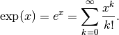
Computes the exponential function,

$\exp(x) = e^x = \sum_{k=0}^{\infty} \frac{x^k}{k!}.$

For complex numbers, the exponential function also satisfies

$\exp(x+yi) = e^x (\cos y + i \sin y).$

Basic examples

Some values of the exponential function:

>>> from mpmath import *
>>> mp.dps = 25; mp.pretty = True
>>> exp(0)
1.0
>>> exp(1)
2.718281828459045235360287
>>> exp(-1)
0.3678794411714423215955238
>>> exp(inf)
+inf
>>> exp(-inf)
0.0

Arguments can be arbitrarily large:

>>> exp(10000)
8.806818225662921587261496e+4342
>>> exp(-10000)
1.135483865314736098540939e-4343

Evaluation is supported for interval arguments via mpmath.iv.exp():

>>> iv.dps = 25; iv.pretty = True
>>> iv.exp([-inf,0])
[0.0, 1.0]
>>> iv.exp([0,1])
[1.0, 2.71828182845904523536028749558]

The exponential function can be evaluated efficiently to arbitrary precision:

>>> mp.dps = 10000
>>> exp(pi)  
23.140692632779269005729...8984304016040616

Functional properties

Numerical verification of Euler’s identity for the complex exponential function:

>>> mp.dps = 15
>>> exp(j*pi)+1
(0.0 + 1.22464679914735e-16j)
>>> chop(exp(j*pi)+1)
0.0

This recovers the coefficients (reciprocal factorials) in the Maclaurin series expansion of exp:

>>> nprint(taylor(exp, 0, 5))
[1.0, 1.0, 0.5, 0.166667, 0.0416667, 0.00833333]

The exponential function is its own derivative and antiderivative:

>>> exp(pi)
23.1406926327793
>>> diff(exp, pi)
23.1406926327793
>>> quad(exp, [-inf, pi])
23.1406926327793

The exponential function can be evaluated using various methods, including direct summation of the series, limits, and solving the defining differential equation:

>>> nsum(lambda k: pi**k/fac(k), [0,inf])
23.1406926327793
>>> limit(lambda k: (1+pi/k)**k, inf)
23.1406926327793
>>> odefun(lambda t, x: x, 0, 1)(pi)
23.1406926327793

`power()`¶

mpmath.power(x, y)¶

Converts $x$ and $y$ to mpmath numbers and evaluates $x^y = \exp(y \log(x))$ :

>>> from mpmath import *
>>> mp.dps = 30; mp.pretty = True
>>> power(2, 0.5)
1.41421356237309504880168872421

This shows the leading few digits of a large Mersenne prime (performing the exact calculation 2**43112609-1 and displaying the result in Python would be very slow):

>>> power(2, 43112609)-1
3.16470269330255923143453723949e+12978188

`expj()`¶

mpmath.expj(x, **kwargs)¶

Convenience function for computing $e^{ix}$ :

>>> from mpmath import *
>>> mp.dps = 25; mp.pretty = True
>>> expj(0)
(1.0 + 0.0j)
>>> expj(-1)
(0.5403023058681397174009366 - 0.8414709848078965066525023j)
>>> expj(j)
(0.3678794411714423215955238 + 0.0j)
>>> expj(1+j)
(0.1987661103464129406288032 + 0.3095598756531121984439128j)

`expjpi()`¶

mpmath.expjpi(x, **kwargs)¶

Convenience function for computing $e^{i \pi x}$ . Evaluation is accurate near zeros (see also cospi(), sinpi()):

>>> from mpmath import *
>>> mp.dps = 25; mp.pretty = True
>>> expjpi(0)
(1.0 + 0.0j)
>>> expjpi(1)
(-1.0 + 0.0j)
>>> expjpi(0.5)
(0.0 + 1.0j)
>>> expjpi(-1)
(-1.0 + 0.0j)
>>> expjpi(j)
(0.04321391826377224977441774 + 0.0j)
>>> expjpi(1+j)
(-0.04321391826377224977441774 + 0.0j)

`expm1()`¶

mpmath.expm1(x)¶

Computes $e^x - 1$ , accurately for small $x$ .

Unlike the expression exp(x) - 1, expm1(x) does not suffer from potentially catastrophic cancellation:

>>> from mpmath import *
>>> mp.dps = 15; mp.pretty = True
>>> exp(1e-10)-1; print(expm1(1e-10))
1.00000008274037e-10
1.00000000005e-10
>>> exp(1e-20)-1; print(expm1(1e-20))
0.0
1.0e-20
>>> 1/(exp(1e-20)-1)
Traceback (most recent call last):
  ...
ZeroDivisionError
>>> 1/expm1(1e-20)
1.0e+20

Evaluation works for extremely tiny values:

>>> expm1(0)
0.0
>>> expm1('1e-10000000')
1.0e-10000000

`powm1()`¶

mpmath.powm1(x, y)¶

Computes $x^y - 1$ , accurately when $x^y$ is very close to 1.

This avoids potentially catastrophic cancellation:

>>> from mpmath import *
>>> mp.dps = 15; mp.pretty = True
>>> power(0.99999995, 1e-10) - 1
0.0
>>> powm1(0.99999995, 1e-10)
-5.00000012791934e-18

Powers exactly equal to 1, and only those powers, yield 0 exactly:

>>> powm1(-j, 4)
(0.0 + 0.0j)
>>> powm1(3, 0)
0.0
>>> powm1(fadd(-1, 1e-100, exact=True), 4)
-4.0e-100

Evaluation works for extremely tiny $y$ :

>>> powm1(2, '1e-100000')
6.93147180559945e-100001
>>> powm1(j, '1e-1000')
(-1.23370055013617e-2000 + 1.5707963267949e-1000j)

Logarithms¶

`log()`¶

mpmath.log(x, b=None)¶

Computes the base- $b$ logarithm of $x$ , $\log_b(x)$ . If $b$ is unspecified, log() computes the natural (base $e$ ) logarithm and is equivalent to ln(). In general, the base $b$ logarithm is defined in terms of the natural logarithm as $\log_b(x) = \ln(x)/\ln(b)$ .

By convention, we take $\log(0) = -\infty$ .

The natural logarithm is real if $x > 0$ and complex if $x < 0$ or if $x$ is complex. The principal branch of the complex logarithm is used, meaning that $\Im(\ln(x)) = -\pi < \arg(x) \le \pi$ .

Examples

Some basic values and limits:

>>> from mpmath import *
>>> mp.dps = 15; mp.pretty = True
>>> log(1)
0.0
>>> log(2)
0.693147180559945
>>> log(1000,10)
3.0
>>> log(4, 16)
0.5
>>> log(j)
(0.0 + 1.5707963267949j)
>>> log(-1)
(0.0 + 3.14159265358979j)
>>> log(0)
-inf
>>> log(inf)
+inf

The natural logarithm is the antiderivative of $1/x$ :

>>> quad(lambda x: 1/x, [1, 5])
1.6094379124341
>>> log(5)
1.6094379124341
>>> diff(log, 10)
0.1

The Taylor series expansion of the natural logarithm around $x = 1$ has coefficients $(-1)^{n+1}/n$ :

>>> nprint(taylor(log, 1, 7))
[0.0, 1.0, -0.5, 0.333333, -0.25, 0.2, -0.166667, 0.142857]

log() supports arbitrary precision evaluation:

>>> mp.dps = 50
>>> log(pi)
1.1447298858494001741434273513530587116472948129153
>>> log(pi, pi**3)
0.33333333333333333333333333333333333333333333333333
>>> mp.dps = 25
>>> log(3+4j)
(1.609437912434100374600759 + 0.9272952180016122324285125j)

`ln()`¶

mpmath.ln(x, **kwargs)¶

Computes the base- $b$ logarithm of $x$ , $\log_b(x)$ . If $b$ is unspecified, log() computes the natural (base $e$ ) logarithm and is equivalent to ln(). In general, the base $b$ logarithm is defined in terms of the natural logarithm as $\log_b(x) = \ln(x)/\ln(b)$ .

By convention, we take $\log(0) = -\infty$ .

The natural logarithm is real if $x > 0$ and complex if $x < 0$ or if $x$ is complex. The principal branch of the complex logarithm is used, meaning that $\Im(\ln(x)) = -\pi < \arg(x) \le \pi$ .

Examples

Some basic values and limits:

>>> from mpmath import *
>>> mp.dps = 15; mp.pretty = True
>>> log(1)
0.0
>>> log(2)
0.693147180559945
>>> log(1000,10)
3.0
>>> log(4, 16)
0.5
>>> log(j)
(0.0 + 1.5707963267949j)
>>> log(-1)
(0.0 + 3.14159265358979j)
>>> log(0)
-inf
>>> log(inf)
+inf

The natural logarithm is the antiderivative of $1/x$ :

>>> quad(lambda x: 1/x, [1, 5])
1.6094379124341
>>> log(5)
1.6094379124341
>>> diff(log, 10)
0.1

The Taylor series expansion of the natural logarithm around $x = 1$ has coefficients $(-1)^{n+1}/n$ :

>>> nprint(taylor(log, 1, 7))
[0.0, 1.0, -0.5, 0.333333, -0.25, 0.2, -0.166667, 0.142857]

log() supports arbitrary precision evaluation:

>>> mp.dps = 50
>>> log(pi)
1.1447298858494001741434273513530587116472948129153
>>> log(pi, pi**3)
0.33333333333333333333333333333333333333333333333333
>>> mp.dps = 25
>>> log(3+4j)
(1.609437912434100374600759 + 0.9272952180016122324285125j)

`log10()`¶

mpmath.log10(x)¶: Computes the base-10 logarithm of $x$ , $\log_{10}(x)$ . log10(x) is equivalent to log(x, 10).

Lambert W function¶

`lambertw()`¶

mpmath.lambertw(z, k=0)¶

The Lambert W function $W(z)$ is defined as the inverse function of $w \exp(w)$ . In other words, the value of $W(z)$ is such that $z = W(z) \exp(W(z))$ for any complex number $z$ .

The Lambert W function is a multivalued function with infinitely many branches $W_k(z)$ , indexed by $k \in \mathbb{Z}$ . Each branch gives a different solution $w$ of the equation $z = w \exp(w)$ . All branches are supported by lambertw():

lambertw(z) gives the principal solution (branch 0)
lambertw(z, k) gives the solution on branch $k$

The Lambert W function has two partially real branches: the principal branch ( $k = 0$ ) is real for real $z > -1/e$ , and the $k = -1$ branch is real for $-1/e < z < 0$ . All branches except $k = 0$ have a logarithmic singularity at $z = 0$ .

The definition, implementation and choice of branches is based on [Corless].

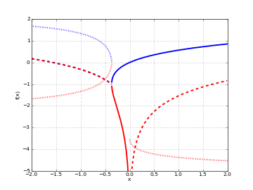
Plots

# Branches 0 and -1 of the Lambert W function
plot([lambertw, lambda x: lambertw(x,-1)], [-2,2], [-5,2], points=2000)

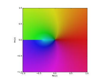
# Principal branch of the Lambert W function W(z)
cplot(lambertw, [-1,1], [-1,1], points=50000)

Basic examples

The Lambert W function is the inverse of $w \exp(w)$ :

>>> from mpmath import *
>>> mp.dps = 25; mp.pretty = True
>>> w = lambertw(1)
>>> w
0.5671432904097838729999687
>>> w*exp(w)
1.0

Any branch gives a valid inverse:

>>> w = lambertw(1, k=3)
>>> w
(-2.853581755409037807206819 + 17.11353553941214591260783j)
>>> w = lambertw(1, k=25)
>>> w
(-5.047020464221569709378686 + 155.4763860949415867162066j)
>>> chop(w*exp(w))
1.0

Applications to equation-solving

The Lambert W function may be used to solve various kinds of equations, such as finding the value of the infinite power tower $z^{z^{z^{\ldots}}}$ :

>>> def tower(z, n):
...     if n == 0:
...         return z
...     return z ** tower(z, n-1)
...
>>> tower(mpf(0.5), 100)
0.6411857445049859844862005
>>> -lambertw(-log(0.5))/log(0.5)
0.6411857445049859844862005

Properties

The Lambert W function grows roughly like the natural logarithm for large arguments:

>>> lambertw(1000); log(1000)
5.249602852401596227126056
6.907755278982137052053974
>>> lambertw(10**100); log(10**100)
224.8431064451185015393731
230.2585092994045684017991

The principal branch of the Lambert W function has a rational Taylor series expansion around $z = 0$ :

>>> nprint(taylor(lambertw, 0, 6), 10)
[0.0, 1.0, -1.0, 1.5, -2.666666667, 5.208333333, -10.8]

Some special values and limits are:

>>> lambertw(0)
0.0
>>> lambertw(1)
0.5671432904097838729999687
>>> lambertw(e)
1.0
>>> lambertw(inf)
+inf
>>> lambertw(0, k=-1)
-inf
>>> lambertw(0, k=3)
-inf
>>> lambertw(inf, k=2)
(+inf + 12.56637061435917295385057j)
>>> lambertw(inf, k=3)
(+inf + 18.84955592153875943077586j)
>>> lambertw(-inf, k=3)
(+inf + 21.9911485751285526692385j)

The $k = 0$ and $k = -1$ branches join at $z = -1/e$ where $W(z) = -1$ for both branches. Since $-1/e$ can only be represented approximately with binary floating-point numbers, evaluating the Lambert W function at this point only gives $-1$ approximately:

>>> lambertw(-1/e, 0)
-0.9999999999998371330228251
>>> lambertw(-1/e, -1)
-1.000000000000162866977175

If $-1/e$ happens to round in the negative direction, there might be a small imaginary part:

>>> mp.dps = 15
>>> lambertw(-1/e)
(-1.0 + 8.22007971483662e-9j)
>>> lambertw(-1/e+eps)
-0.999999966242188

References

[Corless]

Arithmetic-geometric mean¶

`agm()`¶

mpmath.agm(a, b=1)¶

agm(a, b) computes the arithmetic-geometric mean of $a$ and $b$ , defined as the limit of the following iteration:

$a_0 = a b_0 = b a_{n+1} = \frac{a_n+b_n}{2} b_{n+1} = \sqrt{a_n b_n}$

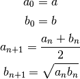
This function can be called with a single argument, computing $\mathrm{agm}(a,1) = \mathrm{agm}(1,a)$ .

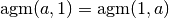Examples

It is a well-known theorem that the geometric mean of two distinct positive numbers is less than the arithmetic mean. It follows that the arithmetic-geometric mean lies between the two means:

>>> from mpmath import *
>>> mp.dps = 15; mp.pretty = True
>>> a = mpf(3)
>>> b = mpf(4)
>>> sqrt(a*b)
3.46410161513775
>>> agm(a,b)
3.48202767635957
>>> (a+b)/2
3.5

The arithmetic-geometric mean is scale-invariant:

>>> agm(10*e, 10*pi)
29.261085515723
>>> 10*agm(e, pi)
29.261085515723

As an order-of-magnitude estimate, $\mathrm{agm}(1,x) \approx x$ for large $x$ :

>>> agm(10**10)
643448704.760133
>>> agm(10**50)
1.34814309345871e+48

For tiny $x$ , $\mathrm{agm}(1,x) \approx -\pi/(2 \log(x/4))$ :

>>> agm('0.01')
0.262166887202249
>>> -pi/2/log('0.0025')
0.262172347753122

The arithmetic-geometric mean can also be computed for complex numbers:

>>> agm(3, 2+j)
(2.51055133276184 + 0.547394054060638j)

The AGM iteration converges very quickly (each step doubles the number of correct digits), so agm() supports efficient high-precision evaluation:

>>> mp.dps = 10000
>>> a = agm(1,2)
>>> str(a)[-10:]
'1679581912'

Mathematical relations

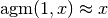
The arithmetic-geometric mean may be used to evaluate the following two parametric definite integrals:

$I_1 = \int_0^{\infty} \frac{1}{\sqrt{(x^2+a^2)(x^2+b^2)}} \,dx I_2 = \int_0^{\pi/2} \frac{1}{\sqrt{a^2 \cos^2(x) + b^2 \sin^2(x)}} \,dx$

We have:

>>> mp.dps = 15
>>> a = 3
>>> b = 4
>>> f1 = lambda x: ((x**2+a**2)*(x**2+b**2))**-0.5
>>> f2 = lambda x: ((a*cos(x))**2 + (b*sin(x))**2)**-0.5
>>> quad(f1, [0, inf])
0.451115405388492
>>> quad(f2, [0, pi/2])
0.451115405388492
>>> pi/(2*agm(a,b))
0.451115405388492

A formula for $\Gamma(1/4)$ :

>>> gamma(0.25)
3.62560990822191
>>> sqrt(2*sqrt(2*pi**3)/agm(1,sqrt(2)))
3.62560990822191

Possible issues

The branch cut chosen for complex $a$ and $b$ is somewhat arbitrary.

Powers and logarithms¶

Nth roots¶

`sqrt()`¶

`hypot()`¶

`cbrt()`¶

`root()`¶

`unitroots()`¶

Exponentiation¶

`exp()`¶

`power()`¶

`expj()`¶

`expjpi()`¶

`expm1()`¶

`powm1()`¶

Logarithms¶

`log()`¶

`ln()`¶

`log10()`¶

Lambert W function¶

`lambertw()`¶

Arithmetic-geometric mean¶

`agm()`¶

Table Of Contents

Previous topic

Next topic

This Page

Navigation

Powers and logarithms¶

Nth roots¶

sqrt()¶

hypot()¶

cbrt()¶

root()¶

unitroots()¶

Exponentiation¶

exp()¶

power()¶

expj()¶

expjpi()¶

expm1()¶

powm1()¶

Logarithms¶

log()¶

ln()¶

log10()¶

Lambert W function¶

lambertw()¶

Arithmetic-geometric mean¶

agm()¶

Table Of Contents

Previous topic

Next topic

This Page

Quick search

Navigation

`sqrt()`¶

`hypot()`¶

`cbrt()`¶

`root()`¶

`unitroots()`¶

`exp()`¶

`power()`¶

`expj()`¶

`expjpi()`¶

`expm1()`¶

`powm1()`¶

`log()`¶

`ln()`¶

`log10()`¶

`lambertw()`¶

`agm()`¶