Bessel functions and related functions

The functions in this section arise as solutions to various differential equations in physics, typically describing wavelike oscillatory behavior or a combination of oscillation and exponential decay or growth. Mathematically, they are special cases of the confluent hypergeometric functions \(\,_0F_1\), \(\,_1F_1\) and \(\,_1F_2\) (see Hypergeometric functions).

Bessel functions

besselj()

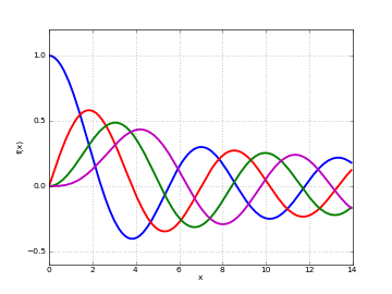
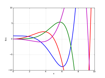
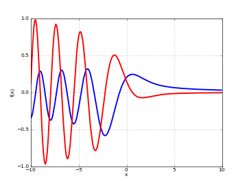
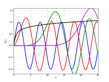
mpmath.besselj(n, x, derivative=0)

besselj(n, x, derivative=0) gives the Bessel function of the first kind \(J_n(x)\). Bessel functions of the first kind are defined as solutions of the differential equation

\[x^2 y'' + x y' + (x^2 - n^2) y = 0\]

which appears, among other things, when solving the radial part of Laplace’s equation in cylindrical coordinates. This equation has two solutions for given \(n\), where the \(J_n\)-function is the solution that is nonsingular at \(x = 0\). For positive integer \(n\), \(J_n(x)\) behaves roughly like a sine (odd \(n\)) or cosine (even \(n\)) multiplied by a magnitude factor that decays slowly as \(x \to \pm\infty\).

Generally, \(J_n\) is a special case of the hypergeometric function \(\,_0F_1\):

\[J_n(x) = \frac{x^n}{2^n \Gamma(n+1)} \,_0F_1\left(n+1,-\frac{x^2}{4}\right)\]

With derivative = \(m \ne 0\), the \(m\)-th derivative

\[\frac{d^m}{dx^m} J_n(x)\]

is computed.

Plots

# Bessel function J_n(x) on the real line for n=0,1,2,3
j0 = lambda x: besselj(0,x)
j1 = lambda x: besselj(1,x)
j2 = lambda x: besselj(2,x)
j3 = lambda x: besselj(3,x)
plot([j0,j1,j2,j3],[0,14])

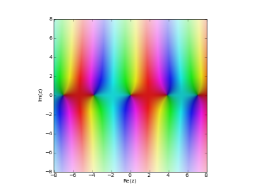
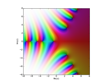
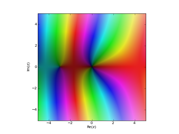
# Bessel function J_n(z) in the complex plane
cplot(lambda z: besselj(1,z), [-8,8], [-8,8], points=50000)

Examples

Evaluation is supported for arbitrary arguments, and at arbitrary precision:

>>> from mpmath import *
>>> mp.dps = 15; mp.pretty = True
>>> besselj(2, 1000)
-0.024777229528606
>>> besselj(4, 0.75)
0.000801070086542314
>>> besselj(2, 1000j)
(-2.48071721019185e+432 + 6.41567059811949e-437j)
>>> mp.dps = 25
>>> besselj(0.75j, 3+4j)
(-2.778118364828153309919653 - 1.5863603889018621585533j)
>>> mp.dps = 50
>>> besselj(1, pi)
0.28461534317975275734531059968613140570981118184947

Arguments may be large:

>>> mp.dps = 25
>>> besselj(0, 10000)
-0.007096160353388801477265164
>>> besselj(0, 10**10)
0.000002175591750246891726859055
>>> besselj(2, 10**100)
7.337048736538615712436929e-51
>>> besselj(2, 10**5*j)
(-3.540725411970948860173735e+43426 + 4.4949812409615803110051e-43433j)

The Bessel functions of the first kind satisfy simple symmetries around \(x = 0\):

>>> mp.dps = 15
>>> nprint([besselj(n,0) for n in range(5)])
[1.0, 0.0, 0.0, 0.0, 0.0]
>>> nprint([besselj(n,pi) for n in range(5)])
[-0.304242, 0.284615, 0.485434, 0.333458, 0.151425]
>>> nprint([besselj(n,-pi) for n in range(5)])
[-0.304242, -0.284615, 0.485434, -0.333458, 0.151425]

Roots of Bessel functions are often used:

>>> nprint([findroot(j0, k) for k in [2, 5, 8, 11, 14]])
[2.40483, 5.52008, 8.65373, 11.7915, 14.9309]
>>> nprint([findroot(j1, k) for k in [3, 7, 10, 13, 16]])
[3.83171, 7.01559, 10.1735, 13.3237, 16.4706]

The roots are not periodic, but the distance between successive roots asymptotically approaches \(2 \pi\). Bessel functions of the first kind have the following normalization:

>>> quadosc(j0, [0, inf], period=2*pi)
1.0
>>> quadosc(j1, [0, inf], period=2*pi)
1.0

For \(n = 1/2\) or \(n = -1/2\), the Bessel function reduces to a trigonometric function:

>>> x = 10
>>> besselj(0.5, x), sqrt(2/(pi*x))*sin(x)
(-0.13726373575505, -0.13726373575505)
>>> besselj(-0.5, x), sqrt(2/(pi*x))*cos(x)
(-0.211708866331398, -0.211708866331398)

Derivatives of any order can be computed (negative orders correspond to integration):

>>> mp.dps = 25
>>> besselj(0, 7.5, 1)
-0.1352484275797055051822405
>>> diff(lambda x: besselj(0,x), 7.5)
-0.1352484275797055051822405
>>> besselj(0, 7.5, 10)
-0.1377811164763244890135677
>>> diff(lambda x: besselj(0,x), 7.5, 10)
-0.1377811164763244890135677
>>> besselj(0,7.5,-1) - besselj(0,3.5,-1)
-0.1241343240399987693521378
>>> quad(j0, [3.5, 7.5])
-0.1241343240399987693521378

Differentiation with a noninteger order gives the fractional derivative in the sense of the Riemann-Liouville differintegral, as computed by differint():

>>> mp.dps = 15
>>> besselj(1, 3.5, 0.75)
-0.385977722939384
>>> differint(lambda x: besselj(1, x), 3.5, 0.75)
-0.385977722939384

mpmath.j0(x)

Computes the Bessel function \(J_0(x)\). See besselj().

mpmath.j1(x)

Computes the Bessel function \(J_1(x)\). See besselj().

bessely()

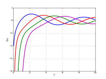
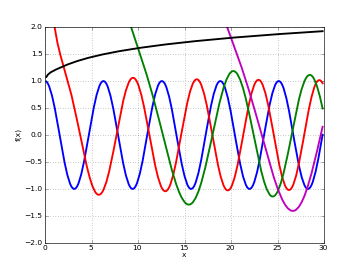
mpmath.bessely(n, x, derivative=0)

bessely(n, x, derivative=0) gives the Bessel function of the second kind,

\[Y_n(x) = \frac{J_n(x) \cos(\pi n) - J_{-n}(x)}{\sin(\pi n)}.\]

For \(n\) an integer, this formula should be understood as a limit. With derivative = \(m \ne 0\), the \(m\)-th derivative

\[\frac{d^m}{dx^m} Y_n(x)\]

is computed.

Plots

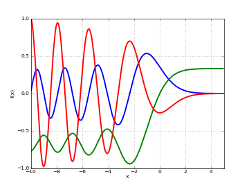
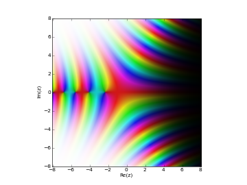
# Bessel function of 2nd kind Y_n(x) on the real line for n=0,1,2,3
y0 = lambda x: bessely(0,x)
y1 = lambda x: bessely(1,x)
y2 = lambda x: bessely(2,x)
y3 = lambda x: bessely(3,x)
plot([y0,y1,y2,y3],[0,10],[-4,1])

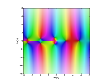
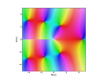
# Bessel function of 2nd kind Y_n(z) in the complex plane
cplot(lambda z: bessely(1,z), [-8,8], [-8,8], points=50000)

Examples

Some values of \(Y_n(x)\):

>>> from mpmath import *
>>> mp.dps = 25; mp.pretty = True
>>> bessely(0,0), bessely(1,0), bessely(2,0)
(-inf, -inf, -inf)
>>> bessely(1, pi)
0.3588729167767189594679827
>>> bessely(0.5, 3+4j)
(9.242861436961450520325216 - 3.085042824915332562522402j)

Arguments may be large:

>>> bessely(0, 10000)
0.00364780555898660588668872
>>> bessely(2.5, 10**50)
-4.8952500412050989295774e-26
>>> bessely(2.5, -10**50)
(0.0 + 4.8952500412050989295774e-26j)

Derivatives and antiderivatives of any order can be computed:

>>> bessely(2, 3.5, 1)
0.3842618820422660066089231
>>> diff(lambda x: bessely(2, x), 3.5)
0.3842618820422660066089231
>>> bessely(0.5, 3.5, 1)
-0.2066598304156764337900417
>>> diff(lambda x: bessely(0.5, x), 3.5)
-0.2066598304156764337900417
>>> diff(lambda x: bessely(2, x), 0.5, 10)
-208173867409.5547350101511
>>> bessely(2, 0.5, 10)
-208173867409.5547350101511
>>> bessely(2, 100.5, 100)
0.02668487547301372334849043
>>> quad(lambda x: bessely(2,x), [1,3])
-1.377046859093181969213262
>>> bessely(2,3,-1) - bessely(2,1,-1)
-1.377046859093181969213262

besseli()

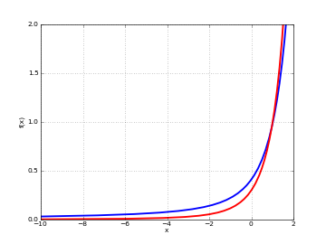
mpmath.besseli(n, x, derivative=0)

besseli(n, x, derivative=0) gives the modified Bessel function of the first kind,

\[I_n(x) = i^{-n} J_n(ix).\]

With derivative = \(m \ne 0\), the \(m\)-th derivative

\[\frac{d^m}{dx^m} I_n(x)\]

is computed.

Plots

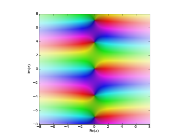
# Modified Bessel function I_n(x) on the real line for n=0,1,2,3
i0 = lambda x: besseli(0,x)
i1 = lambda x: besseli(1,x)
i2 = lambda x: besseli(2,x)
i3 = lambda x: besseli(3,x)
plot([i0,i1,i2,i3],[0,5],[0,5])

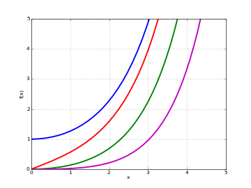
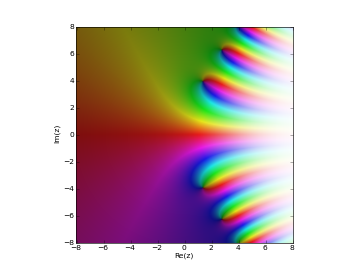
# Modified Bessel function I_n(z) in the complex plane
cplot(lambda z: besseli(1,z), [-8,8], [-8,8], points=50000)

Examples

Some values of \(I_n(x)\):

>>> from mpmath import *
>>> mp.dps = 25; mp.pretty = True
>>> besseli(0,0)
1.0
>>> besseli(1,0)
0.0
>>> besseli(0,1)
1.266065877752008335598245
>>> besseli(3.5, 2+3j)
(-0.2904369752642538144289025 - 0.4469098397654815837307006j)

Arguments may be large:

>>> besseli(2, 1000)
2.480717210191852440616782e+432
>>> besseli(2, 10**10)
4.299602851624027900335391e+4342944813
>>> besseli(2, 6000+10000j)
(-2.114650753239580827144204e+2603 + 4.385040221241629041351886e+2602j)

For integers \(n\), the following integral representation holds:

>>> mp.dps = 15
>>> n = 3
>>> x = 2.3
>>> quad(lambda t: exp(x*cos(t))*cos(n*t), [0,pi])/pi
0.349223221159309
>>> besseli(n,x)
0.349223221159309

Derivatives and antiderivatives of any order can be computed:

>>> mp.dps = 25
>>> besseli(2, 7.5, 1)
195.8229038931399062565883
>>> diff(lambda x: besseli(2,x), 7.5)
195.8229038931399062565883
>>> besseli(2, 7.5, 10)
153.3296508971734525525176
>>> diff(lambda x: besseli(2,x), 7.5, 10)
153.3296508971734525525176
>>> besseli(2,7.5,-1) - besseli(2,3.5,-1)
202.5043900051930141956876
>>> quad(lambda x: besseli(2,x), [3.5, 7.5])
202.5043900051930141956876

besselk()

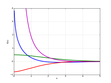
mpmath.besselk(n, x)

besselk(n, x) gives the modified Bessel function of the second kind,

\[K_n(x) = \frac{\pi}{2} \frac{I_{-n}(x)-I_{n}(x)}{\sin(\pi n)}\]

For \(n\) an integer, this formula should be understood as a limit.

Plots

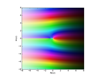
# Modified Bessel function of 2nd kind K_n(x) on the real line for n=0,1,2,3
k0 = lambda x: besselk(0,x)
k1 = lambda x: besselk(1,x)
k2 = lambda x: besselk(2,x)
k3 = lambda x: besselk(3,x)
plot([k0,k1,k2,k3],[0,8],[0,5])

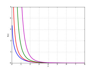
# Modified Bessel function of 2nd kind K_n(z) in the complex plane
cplot(lambda z: besselk(1,z), [-8,8], [-8,8], points=50000)

Examples

Evaluation is supported for arbitrary complex arguments:

>>> from mpmath import *
>>> mp.dps = 25; mp.pretty = True
>>> besselk(0,1)
0.4210244382407083333356274
>>> besselk(0, -1)
(0.4210244382407083333356274 - 3.97746326050642263725661j)
>>> besselk(3.5, 2+3j)
(-0.02090732889633760668464128 + 0.2464022641351420167819697j)
>>> besselk(2+3j, 0.5)
(0.9615816021726349402626083 + 0.1918250181801757416908224j)

Arguments may be large:

>>> besselk(0, 100)
4.656628229175902018939005e-45
>>> besselk(1, 10**6)
4.131967049321725588398296e-434298
>>> besselk(1, 10**6*j)
(0.001140348428252385844876706 - 0.0005200017201681152909000961j)
>>> besselk(4.5, fmul(10**50, j, exact=True))
(1.561034538142413947789221e-26 + 1.243554598118700063281496e-25j)

The point \(x = 0\) is a singularity (logarithmic if \(n = 0\)):

>>> besselk(0,0)
+inf
>>> besselk(1,0)
+inf
>>> for n in range(-4, 5):
...     print(besselk(n, '1e-1000'))
...
4.8e+4001
8.0e+3000
2.0e+2000
1.0e+1000
2302.701024509704096466802
1.0e+1000
2.0e+2000
8.0e+3000
4.8e+4001

Bessel function zeros

besseljzero()

mpmath.besseljzero(v, m, derivative=0)

For a real order \(\nu \ge 0\) and a positive integer \(m\), returns \(j_{\nu,m}\), the \(m\)-th positive zero of the Bessel function of the first kind \(J_{\nu}(z)\) (see besselj()). Alternatively, with derivative=1, gives the first nonnegative simple zero \(j'_{\nu,m}\) of \(J'_{\nu}(z)\).

The indexing convention is that used by Abramowitz & Stegun and the DLMF. Note the special case \(j'_{0,1} = 0\), while all other zeros are positive. In effect, only simple zeros are counted (all zeros of Bessel functions are simple except possibly \(z = 0\)) and \(j_{\nu,m}\) becomes a monotonic function of both \(\nu\) and \(m\).

The zeros are interlaced according to the inequalities

\[ \begin{align}\begin{aligned}j'_{\nu,k} < j_{\nu,k} < j'_{\nu,k+1}\\j_{\nu,1} < j_{\nu+1,2} < j_{\nu,2} < j_{\nu+1,2} < j_{\nu,3} < \cdots\end{aligned}\end{align} \]

Examples

Initial zeros of the Bessel functions \(J_0(z), J_1(z), J_2(z)\):

>>> from mpmath import *
>>> mp.dps = 25; mp.pretty = True
>>> besseljzero(0,1); besseljzero(0,2); besseljzero(0,3)
2.404825557695772768621632
5.520078110286310649596604
8.653727912911012216954199
>>> besseljzero(1,1); besseljzero(1,2); besseljzero(1,3)
3.831705970207512315614436
7.01558666981561875353705
10.17346813506272207718571
>>> besseljzero(2,1); besseljzero(2,2); besseljzero(2,3)
5.135622301840682556301402
8.417244140399864857783614
11.61984117214905942709415

Initial zeros of \(J'_0(z), J'_1(z), J'_2(z)\):

0.0
3.831705970207512315614436
7.01558666981561875353705
>>> besseljzero(1,1,1); besseljzero(1,2,1); besseljzero(1,3,1)
1.84118378134065930264363
5.331442773525032636884016
8.536316366346285834358961
>>> besseljzero(2,1,1); besseljzero(2,2,1); besseljzero(2,3,1)
3.054236928227140322755932
6.706133194158459146634394
9.969467823087595793179143

Zeros with large index:

>>> besseljzero(0,100); besseljzero(0,1000); besseljzero(0,10000)
313.3742660775278447196902
3140.807295225078628895545
31415.14114171350798533666
>>> besseljzero(5,100); besseljzero(5,1000); besseljzero(5,10000)
321.1893195676003157339222
3148.657306813047523500494
31422.9947255486291798943
>>> besseljzero(0,100,1); besseljzero(0,1000,1); besseljzero(0,10000,1)
311.8018681873704508125112
3139.236339643802482833973
31413.57032947022399485808

Zeros of functions with large order:

>>> besseljzero(50,1)
57.11689916011917411936228
>>> besseljzero(50,2)
62.80769876483536093435393
>>> besseljzero(50,100)
388.6936600656058834640981
>>> besseljzero(50,1,1)
52.99764038731665010944037
>>> besseljzero(50,2,1)
60.02631933279942589882363
>>> besseljzero(50,100,1)
387.1083151608726181086283

Zeros of functions with fractional order:

>>> besseljzero(0.5,1); besseljzero(1.5,1); besseljzero(2.25,4)
3.141592653589793238462643
4.493409457909064175307881
15.15657692957458622921634

Both \(J_{\nu}(z)\) and \(J'_{\nu}(z)\) can be expressed as infinite products over their zeros:

>>> v,z = 2, mpf(1)
>>> (z/2)**v/gamma(v+1) * \
...     nprod(lambda k: 1-(z/besseljzero(v,k))**2, [1,inf])
...
0.1149034849319004804696469
>>> besselj(v,z)
0.1149034849319004804696469
>>> (z/2)**(v-1)/2/gamma(v) * \
...     nprod(lambda k: 1-(z/besseljzero(v,k,1))**2, [1,inf])
...
0.2102436158811325550203884
>>> besselj(v,z,1)
0.2102436158811325550203884

besselyzero()

mpmath.besselyzero(v, m, derivative=0)

For a real order \(\nu \ge 0\) and a positive integer \(m\), returns \(y_{\nu,m}\), the \(m\)-th positive zero of the Bessel function of the second kind \(Y_{\nu}(z)\) (see bessely()). Alternatively, with derivative=1, gives the first positive zero \(y'_{\nu,m}\) of \(Y'_{\nu}(z)\).

The zeros are interlaced according to the inequalities

\[ \begin{align}\begin{aligned}y_{\nu,k} < y'_{\nu,k} < y_{\nu,k+1}\\y_{\nu,1} < y_{\nu+1,2} < y_{\nu,2} < y_{\nu+1,2} < y_{\nu,3} < \cdots\end{aligned}\end{align} \]

Examples

Initial zeros of the Bessel functions \(Y_0(z), Y_1(z), Y_2(z)\):

>>> from mpmath import *
>>> mp.dps = 25; mp.pretty = True
>>> besselyzero(0,1); besselyzero(0,2); besselyzero(0,3)
0.8935769662791675215848871
3.957678419314857868375677
7.086051060301772697623625
>>> besselyzero(1,1); besselyzero(1,2); besselyzero(1,3)
2.197141326031017035149034
5.429681040794135132772005
8.596005868331168926429606
>>> besselyzero(2,1); besselyzero(2,2); besselyzero(2,3)
3.384241767149593472701426
6.793807513268267538291167
10.02347797936003797850539

Initial zeros of \(Y'_0(z), Y'_1(z), Y'_2(z)\):

>>> besselyzero(0,1,1); besselyzero(0,2,1); besselyzero(0,3,1)
2.197141326031017035149034
5.429681040794135132772005
8.596005868331168926429606
>>> besselyzero(1,1,1); besselyzero(1,2,1); besselyzero(1,3,1)
3.683022856585177699898967
6.941499953654175655751944
10.12340465543661307978775
>>> besselyzero(2,1,1); besselyzero(2,2,1); besselyzero(2,3,1)
5.002582931446063945200176
8.350724701413079526349714
11.57419546521764654624265

Zeros with large index:

>>> besselyzero(0,100); besselyzero(0,1000); besselyzero(0,10000)
311.8034717601871549333419
3139.236498918198006794026
31413.57034538691205229188
>>> besselyzero(5,100); besselyzero(5,1000); besselyzero(5,10000)
319.6183338562782156235062
3147.086508524556404473186
31421.42392920214673402828
>>> besselyzero(0,100,1); besselyzero(0,1000,1); besselyzero(0,10000,1)
313.3726705426359345050449
3140.807136030340213610065
31415.14112579761578220175

Zeros of functions with large order:

>>> besselyzero(50,1)
53.50285882040036394680237
>>> besselyzero(50,2)
60.11244442774058114686022
>>> besselyzero(50,100)
387.1096509824943957706835
>>> besselyzero(50,1,1)
56.96290427516751320063605
>>> besselyzero(50,2,1)
62.74888166945933944036623
>>> besselyzero(50,100,1)
388.6923300548309258355475

Zeros of functions with fractional order:

>>> besselyzero(0.5,1); besselyzero(1.5,1); besselyzero(2.25,4)
1.570796326794896619231322
2.798386045783887136720249
13.56721208770735123376018

Hankel functions

hankel1()

mpmath.hankel1(n, x)

hankel1(n,x) computes the Hankel function of the first kind, which is the complex combination of Bessel functions given by

\[H_n^{(1)}(x) = J_n(x) + i Y_n(x).\]

Plots

# Hankel function H1_n(x) on the real line for n=0,1,2,3
h0 = lambda x: hankel1(0,x)
h1 = lambda x: hankel1(1,x)
h2 = lambda x: hankel1(2,x)
h3 = lambda x: hankel1(3,x)
plot([h0,h1,h2,h3],[0,6],[-2,1])

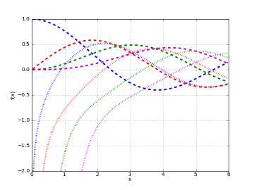
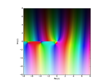
# Hankel function H1_n(z) in the complex plane
cplot(lambda z: hankel1(1,z), [-8,8], [-8,8], points=50000)

Examples

The Hankel function is generally complex-valued:

>>> from mpmath import *
>>> mp.dps = 25; mp.pretty = True
>>> hankel1(2, pi)
(0.4854339326315091097054957 - 0.0999007139290278787734903j)
>>> hankel1(3.5, pi)
(0.2340002029630507922628888 - 0.6419643823412927142424049j)

hankel2()

mpmath.hankel2(n, x)

hankel2(n,x) computes the Hankel function of the second kind, which is the complex combination of Bessel functions given by

\[H_n^{(2)}(x) = J_n(x) - i Y_n(x).\]

Plots

# Hankel function H2_n(x) on the real line for n=0,1,2,3
h0 = lambda x: hankel2(0,x)
h1 = lambda x: hankel2(1,x)
h2 = lambda x: hankel2(2,x)
h3 = lambda x: hankel2(3,x)
plot([h0,h1,h2,h3],[0,6],[-1,2])

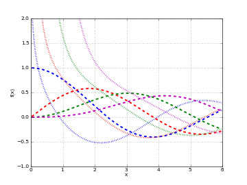
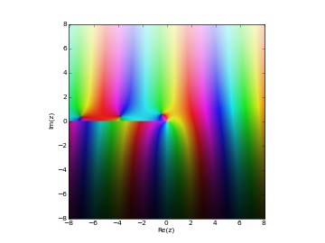
# Hankel function H2_n(z) in the complex plane
cplot(lambda z: hankel2(1,z), [-8,8], [-8,8], points=50000)

Examples

The Hankel function is generally complex-valued:

>>> from mpmath import *
>>> mp.dps = 25; mp.pretty = True
>>> hankel2(2, pi)
(0.4854339326315091097054957 + 0.0999007139290278787734903j)
>>> hankel2(3.5, pi)
(0.2340002029630507922628888 + 0.6419643823412927142424049j)

Kelvin functions

ber()

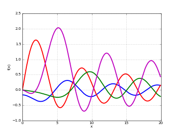
mpmath.ber(n, z, **kwargs)

Computes the Kelvin function ber, which for real arguments gives the real part of the Bessel J function of a rotated argument

\[J_n\left(x e^{3\pi i/4}\right) = \mathrm{ber}_n(x) + i \mathrm{bei}_n(x).\]

The imaginary part is given by bei().

Plots

# Kelvin functions ber_n(x) and bei_n(x) on the real line for n=0,2
f0 = lambda x: ber(0,x)
f1 = lambda x: bei(0,x)
f2 = lambda x: ber(2,x)
f3 = lambda x: bei(2,x)
plot([f0,f1,f2,f3],[0,10],[-10,10])

Examples

Verifying the defining relation:

>>> from mpmath import *
>>> mp.dps = 25; mp.pretty = True
>>> n, x = 2, 3.5
>>> ber(n,x)
1.442338852571888752631129
>>> bei(n,x)
-0.948359035324558320217678
>>> besselj(n, x*root(1,8,3))
(1.442338852571888752631129 - 0.948359035324558320217678j)

The ber and bei functions are also defined by analytic continuation for complex arguments:

>>> ber(1+j, 2+3j)
(4.675445984756614424069563 - 15.84901771719130765656316j)
>>> bei(1+j, 2+3j)
(15.83886679193707699364398 + 4.684053288183046528703611j)

bei()

mpmath.bei(n, z, **kwargs)

Computes the Kelvin function bei, which for real arguments gives the imaginary part of the Bessel J function of a rotated argument. See ber().

ker()

mpmath.ker(n, z, **kwargs)

Computes the Kelvin function ker, which for real arguments gives the real part of the (rescaled) Bessel K function of a rotated argument

\[e^{-\pi i/2} K_n\left(x e^{3\pi i/4}\right) = \mathrm{ker}_n(x) + i \mathrm{kei}_n(x).\]

The imaginary part is given by kei().

Plots

# Kelvin functions ker_n(x) and kei_n(x) on the real line for n=0,2
f0 = lambda x: ker(0,x)
f1 = lambda x: kei(0,x)
f2 = lambda x: ker(2,x)
f3 = lambda x: kei(2,x)
plot([f0,f1,f2,f3],[0,5],[-1,4])

Examples

Verifying the defining relation:

>>> from mpmath import *
>>> mp.dps = 25; mp.pretty = True
>>> n, x = 2, 4.5
>>> ker(n,x)
0.02542895201906369640249801
>>> kei(n,x)
-0.02074960467222823237055351
>>> exp(-n*pi*j/2) * besselk(n, x*root(1,8,1))
(0.02542895201906369640249801 - 0.02074960467222823237055351j)

The ker and kei functions are also defined by analytic continuation for complex arguments:

>>> ker(1+j, 3+4j)
(1.586084268115490421090533 - 2.939717517906339193598719j)
>>> kei(1+j, 3+4j)
(-2.940403256319453402690132 - 1.585621643835618941044855j)

kei()

mpmath.kei(n, z, **kwargs)

Computes the Kelvin function kei, which for real arguments gives the imaginary part of the (rescaled) Bessel K function of a rotated argument. See ker().

Struve functions

struveh()

mpmath.struveh(n, z, **kwargs)

Gives the Struve function

\[\,\mathbf{H}_n(z) = \sum_{k=0}^\infty \frac{(-1)^k}{\Gamma(k+\frac{3}{2}) \Gamma(k+n+\frac{3}{2})} {\left({\frac{z}{2}}\right)}^{2k+n+1}\]

which is a solution to the Struve differential equation

\[z^2 f''(z) + z f'(z) + (z^2-n^2) f(z) = \frac{2 z^{n+1}}{\pi (2n-1)!!}.\]

Examples

Evaluation for arbitrary real and complex arguments:

>>> from mpmath import *
>>> mp.dps = 25; mp.pretty = True
>>> struveh(0, 3.5)
0.3608207733778295024977797
>>> struveh(-1, 10)
-0.255212719726956768034732
>>> struveh(1, -100.5)
0.5819566816797362287502246
>>> struveh(2.5, 10000000000000)
3153915652525200060.308937
>>> struveh(2.5, -10000000000000)
(0.0 - 3153915652525200060.308937j)
>>> struveh(1+j, 1000000+4000000j)
(-3.066421087689197632388731e+1737173 - 1.596619701076529803290973e+1737173j)

A Struve function of half-integer order is elementary; for example:

>>> z = 3
>>> struveh(0.5, 3)
0.9167076867564138178671595
>>> sqrt(2/(pi*z))*(1-cos(z))
0.9167076867564138178671595

Numerically verifying the differential equation:

>>> z = mpf(4.5)
>>> n = 3
>>> f = lambda z: struveh(n,z)
>>> lhs = z**2*diff(f,z,2) + z*diff(f,z) + (z**2-n**2)*f(z)
>>> rhs = 2*z**(n+1)/fac2(2*n-1)/pi
>>> lhs
17.40359302709875496632744
>>> rhs
17.40359302709875496632744

struvel()

mpmath.struvel(n, z, **kwargs)

Gives the modified Struve function

\[\,\mathbf{L}_n(z) = -i e^{-n\pi i/2} \mathbf{H}_n(i z)\]

which solves to the modified Struve differential equation

\[z^2 f''(z) + z f'(z) - (z^2+n^2) f(z) = \frac{2 z^{n+1}}{\pi (2n-1)!!}.\]

Examples

Evaluation for arbitrary real and complex arguments:

>>> from mpmath import *
>>> mp.dps = 25; mp.pretty = True
>>> struvel(0, 3.5)
7.180846515103737996249972
>>> struvel(-1, 10)
2670.994904980850550721511
>>> struvel(1, -100.5)
1.757089288053346261497686e+42
>>> struvel(2.5, 10000000000000)
4.160893281017115450519948e+4342944819025
>>> struvel(2.5, -10000000000000)
(0.0 - 4.160893281017115450519948e+4342944819025j)
>>> struvel(1+j, 700j)
(-0.1721150049480079451246076 + 0.1240770953126831093464055j)
>>> struvel(1+j, 1000000+4000000j)
(-2.973341637511505389128708e+434290 - 5.164633059729968297147448e+434290j)

Numerically verifying the differential equation:

>>> z = mpf(3.5)
>>> n = 3
>>> f = lambda z: struvel(n,z)
>>> lhs = z**2*diff(f,z,2) + z*diff(f,z) - (z**2+n**2)*f(z)
>>> rhs = 2*z**(n+1)/fac2(2*n-1)/pi
>>> lhs
6.368850306060678353018165
>>> rhs
6.368850306060678353018165

Anger-Weber functions

angerj()

mpmath.angerj(v, z, **kwargs)

Gives the Anger function

\[\mathbf{J}_{\nu}(z) = \frac{1}{\pi} \int_0^{\pi} \cos(\nu t - z \sin t) dt\]

which is an entire function of both the parameter \(\nu\) and the argument \(z\). It solves the inhomogeneous Bessel differential equation

\[f''(z) + \frac{1}{z}f'(z) + \left(1-\frac{\nu^2}{z^2}\right) f(z) = \frac{(z-\nu)}{\pi z^2} \sin(\pi \nu).\]

Examples

Evaluation for real and complex parameter and argument:

>>> from mpmath import *
>>> mp.dps = 25; mp.pretty = True
>>> angerj(2,3)
0.4860912605858910769078311
>>> angerj(-3+4j, 2+5j)
(-5033.358320403384472395612 + 585.8011892476145118551756j)
>>> angerj(3.25, 1e6j)
(4.630743639715893346570743e+434290 - 1.117960409887505906848456e+434291j)
>>> angerj(-1.5, 1e6)
0.0002795719747073879393087011

The Anger function coincides with the Bessel J-function when \(\nu\) is an integer:

>>> angerj(1,3); besselj(1,3)
0.3390589585259364589255146
0.3390589585259364589255146
>>> angerj(1.5,3); besselj(1.5,3)
0.4088969848691080859328847
0.4777182150870917715515015

Verifying the differential equation:

>>> v,z = mpf(2.25), 0.75
>>> f = lambda z: angerj(v,z)
>>> diff(f,z,2) + diff(f,z)/z + (1-(v/z)**2)*f(z)
-0.6002108774380707130367995
>>> (z-v)/(pi*z**2) * sinpi(v)
-0.6002108774380707130367995

Verifying the integral representation:

>>> angerj(v,z)
0.1145380759919333180900501
>>> quad(lambda t: cos(v*t-z*sin(t))/pi, [0,pi])
0.1145380759919333180900501

References

1. [DLMF] section 11.10: Anger-Weber Functions

webere()

mpmath.webere(v, z, **kwargs)

Gives the Weber function

\[\mathbf{E}_{\nu}(z) = \frac{1}{\pi} \int_0^{\pi} \sin(\nu t - z \sin t) dt\]

which is an entire function of both the parameter \(\nu\) and the argument \(z\). It solves the inhomogeneous Bessel differential equation

\[f''(z) + \frac{1}{z}f'(z) + \left(1-\frac{\nu^2}{z^2}\right) f(z) = -\frac{1}{\pi z^2} (z+\nu+(z-\nu)\cos(\pi \nu)).\]

Examples

Evaluation for real and complex parameter and argument:

>>> from mpmath import *
>>> mp.dps = 25; mp.pretty = True
>>> webere(2,3)
-0.1057668973099018425662646
>>> webere(-3+4j, 2+5j)
(-585.8081418209852019290498 - 5033.314488899926921597203j)
>>> webere(3.25, 1e6j)
(-1.117960409887505906848456e+434291 - 4.630743639715893346570743e+434290j)
>>> webere(3.25, 1e6)
-0.00002812518265894315604914453

Up to addition of a rational function of \(z\), the Weber function coincides with the Struve H-function when \(\nu\) is an integer:

>>> webere(1,3); 2/pi-struveh(1,3)
-0.3834897968188690177372881
-0.3834897968188690177372881
>>> webere(5,3); 26/(35*pi)-struveh(5,3)
0.2009680659308154011878075
0.2009680659308154011878075

Verifying the differential equation:

>>> v,z = mpf(2.25), 0.75
>>> f = lambda z: webere(v,z)
>>> diff(f,z,2) + diff(f,z)/z + (1-(v/z)**2)*f(z)
-1.097441848875479535164627
>>> -(z+v+(z-v)*cospi(v))/(pi*z**2)
-1.097441848875479535164627

Verifying the integral representation:

>>> webere(v,z)
0.1486507351534283744485421
>>> quad(lambda t: sin(v*t-z*sin(t))/pi, [0,pi])
0.1486507351534283744485421

References

1. [DLMF] section 11.10: Anger-Weber Functions

Lommel functions

lommels1()

mpmath.lommels1(u, v, z, **kwargs)

Gives the Lommel function \(s_{\mu,\nu}\) or \(s^{(1)}_{\mu,\nu}\)

\[s_{\mu,\nu}(z) = \frac{z^{\mu+1}}{(\mu-\nu+1)(\mu+\nu+1)} \,_1F_2\left(1; \frac{\mu-\nu+3}{2}, \frac{\mu+\nu+3}{2}; -\frac{z^2}{4} \right)\]

which solves the inhomogeneous Bessel equation

\[z^2 f''(z) + z f'(z) + (z^2-\nu^2) f(z) = z^{\mu+1}.\]

A second solution is given by lommels2().

Plots

# Lommel function s_(u,v)(x) on the real line for a few different u,v
f1 = lambda x: lommels1(-1,2.5,x)
f2 = lambda x: lommels1(0,0.5,x)
f3 = lambda x: lommels1(0,6,x)
f4 = lambda x: lommels1(0.5,3,x)
plot([f1,f2,f3,f4], [0,20])

Examples

An integral representation:

>>> from mpmath import *
>>> mp.dps = 25; mp.pretty = True
>>> u,v,z = 0.25, 0.125, mpf(0.75)
>>> lommels1(u,v,z)
0.4276243877565150372999126
>>> (bessely(v,z)*quad(lambda t: t**u*besselj(v,t), [0,z]) - \
...  besselj(v,z)*quad(lambda t: t**u*bessely(v,t), [0,z]))*(pi/2)
0.4276243877565150372999126

A special value:

>>> lommels1(v,v,z)
0.5461221367746048054932553
>>> gamma(v+0.5)*sqrt(pi)*power(2,v-1)*struveh(v,z)
0.5461221367746048054932553

Verifying the differential equation:

>>> f = lambda z: lommels1(u,v,z)
>>> z**2*diff(f,z,2) + z*diff(f,z) + (z**2-v**2)*f(z)
0.6979536443265746992059141
>>> z**(u+1)
0.6979536443265746992059141

References

1. [GradshteynRyzhik]
2. [Weisstein] http://mathworld.wolfram.com/LommelFunction.html

lommels2()

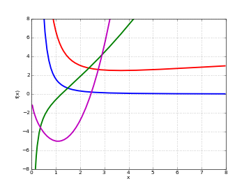
mpmath.lommels2(u, v, z, **kwargs)

Gives the second Lommel function \(S_{\mu,\nu}\) or \(s^{(2)}_{\mu,\nu}\)

\[ \begin{align}\begin{aligned}S_{\mu,\nu}(z) = s_{\mu,\nu}(z) + 2^{\mu-1} \Gamma\left(\tfrac{1}{2}(\mu-\nu+1)\right) \Gamma\left(\tfrac{1}{2}(\mu+\nu+1)\right) \times\\ \left[\sin(\tfrac{1}{2}(\mu-\nu)\pi) J_{\nu}(z) - \cos(\tfrac{1}{2}(\mu-\nu)\pi) Y_{\nu}(z) \right]\end{aligned}\end{align} \]

which solves the same differential equation as lommels1().

Plots

# Lommel function S_(u,v)(x) on the real line for a few different u,v
f1 = lambda x: lommels2(-1,2.5,x)
f2 = lambda x: lommels2(1.5,2,x)
f3 = lambda x: lommels2(2.5,1,x)
f4 = lambda x: lommels2(3.5,-0.5,x)
plot([f1,f2,f3,f4], [0,8], [-8,8])

Examples

For large \(|z|\), \(S_{\mu,\nu} \sim z^{\mu-1}\):

>>> from mpmath import *
>>> mp.dps = 25; mp.pretty = True
>>> lommels2(10,2,30000)
1.968299831601008419949804e+40
>>> power(30000,9)
1.9683e+40

A special value:

>>> u,v,z = 0.5, 0.125, mpf(0.75)
>>> lommels2(v,v,z)
0.9589683199624672099969765
>>> (struveh(v,z)-bessely(v,z))*power(2,v-1)*sqrt(pi)*gamma(v+0.5)
0.9589683199624672099969765

Verifying the differential equation:

>>> f = lambda z: lommels2(u,v,z)
>>> z**2*diff(f,z,2) + z*diff(f,z) + (z**2-v**2)*f(z)
0.6495190528383289850727924
>>> z**(u+1)
0.6495190528383289850727924

References

1. [GradshteynRyzhik]
2. [Weisstein] http://mathworld.wolfram.com/LommelFunction.html

Airy and Scorer functions

airyai()

mpmath.airyai(z, derivative=0, **kwargs)

Computes the Airy function \(\operatorname{Ai}(z)\), which is the solution of the Airy differential equation \(f''(z) - z f(z) = 0\) with initial conditions

\[ \begin{align}\begin{aligned}\operatorname{Ai}(0) = \frac{1}{3^{2/3}\Gamma\left(\frac{2}{3}\right)}\\\operatorname{Ai}'(0) = -\frac{1}{3^{1/3}\Gamma\left(\frac{1}{3}\right)}.\end{aligned}\end{align} \]

Other common ways of defining the Ai-function include integrals such as

\[ \begin{align}\begin{aligned}\operatorname{Ai}(x) = \frac{1}{\pi} \int_0^{\infty} \cos\left(\frac{1}{3}t^3+xt\right) dt \qquad x \in \mathbb{R}\\\operatorname{Ai}(z) = \frac{\sqrt{3}}{2\pi} \int_0^{\infty} \exp\left(-\frac{t^3}{3}-\frac{z^3}{3t^3}\right) dt.\end{aligned}\end{align} \]

The Ai-function is an entire function with a turning point, behaving roughly like a slowly decaying sine wave for \(z < 0\) and like a rapidly decreasing exponential for \(z > 0\). A second solution of the Airy differential equation is given by \(\operatorname{Bi}(z)\) (see airybi()).

Optionally, with derivative=alpha, airyai() can compute the \(\alpha\)-th order fractional derivative with respect to \(z\). For \(\alpha = n = 1,2,3,\ldots\) this gives the derivative \(\operatorname{Ai}^{(n)}(z)\), and for \(\alpha = -n = -1,-2,-3,\ldots\) this gives the \(n\)-fold iterated integral

\[ \begin{align}\begin{aligned}f_0(z) = \operatorname{Ai}(z)\\f_n(z) = \int_0^z f_{n-1}(t) dt.\end{aligned}\end{align} \]

The Ai-function has infinitely many zeros, all located along the negative half of the real axis. They can be computed with airyaizero().

Plots

# Airy function Ai(x), Ai'(x) and int_0^x Ai(t) dt on the real line
f = airyai
f_diff = lambda z: airyai(z, derivative=1)
f_int = lambda z: airyai(z, derivative=-1)
plot([f, f_diff, f_int], [-10,5])

# Airy function Ai(z) in the complex plane
cplot(airyai, [-8,8], [-8,8], points=50000)

Basic examples

Limits and values include:

>>> from mpmath import *
>>> mp.dps = 25; mp.pretty = True
>>> airyai(0); 1/(power(3,'2/3')*gamma('2/3'))
0.3550280538878172392600632
0.3550280538878172392600632
>>> airyai(1)
0.1352924163128814155241474
>>> airyai(-1)
0.5355608832923521187995166
>>> airyai(inf); airyai(-inf)
0.0
0.0

Evaluation is supported for large magnitudes of the argument:

>>> airyai(-100)
0.1767533932395528780908311
>>> airyai(100)
2.634482152088184489550553e-291
>>> airyai(50+50j)
(-5.31790195707456404099817e-68 - 1.163588003770709748720107e-67j)
>>> airyai(-50+50j)
(1.041242537363167632587245e+158 + 3.347525544923600321838281e+157j)

Huge arguments are also fine:

>>> airyai(10**10)
1.162235978298741779953693e-289529654602171
>>> airyai(-10**10)
0.0001736206448152818510510181
>>> w = airyai(10**10*(1+j))
>>> w.real
5.711508683721355528322567e-186339621747698
>>> w.imag
1.867245506962312577848166e-186339621747697

The first root of the Ai-function is:

>>> findroot(airyai, -2)
-2.338107410459767038489197
>>> airyaizero(1)
-2.338107410459767038489197

Properties and relations

Verifying the Airy differential equation:

>>> for z in [-3.4, 0, 2.5, 1+2j]:
...     chop(airyai(z,2) - z*airyai(z))
...
0.0
0.0
0.0
0.0

The first few terms of the Taylor series expansion around \(z = 0\) (every third term is zero):

>>> nprint(taylor(airyai, 0, 5))
[0.355028, -0.258819, 0.0, 0.0591713, -0.0215683, 0.0]

The Airy functions satisfy the Wronskian relation \(\operatorname{Ai}(z) \operatorname{Bi}'(z) - \operatorname{Ai}'(z) \operatorname{Bi}(z) = 1/\pi\):

>>> z = -0.5
>>> airyai(z)*airybi(z,1) - airyai(z,1)*airybi(z)
0.3183098861837906715377675
>>> 1/pi
0.3183098861837906715377675

The Airy functions can be expressed in terms of Bessel functions of order \(\pm 1/3\). For \(\Re[z] \le 0\), we have:

>>> z = -3
>>> airyai(z)
-0.3788142936776580743472439
>>> y = 2*power(-z,'3/2')/3
>>> (sqrt(-z) * (besselj('1/3',y) + besselj('-1/3',y)))/3
-0.3788142936776580743472439

Derivatives and integrals

Derivatives of the Ai-function (directly and using diff()):

>>> airyai(-3,1); diff(airyai,-3)
0.3145837692165988136507873
0.3145837692165988136507873
>>> airyai(-3,2); diff(airyai,-3,2)
1.136442881032974223041732
1.136442881032974223041732
>>> airyai(1000,1); diff(airyai,1000)
-2.943133917910336090459748e-9156
-2.943133917910336090459748e-9156

Several derivatives at \(z = 0\):

>>> airyai(0,0); airyai(0,1); airyai(0,2)
0.3550280538878172392600632
-0.2588194037928067984051836
0.0
>>> airyai(0,3); airyai(0,4); airyai(0,5)
0.3550280538878172392600632
-0.5176388075856135968103671
0.0
>>> airyai(0,15); airyai(0,16); airyai(0,17)
1292.30211615165475090663
-3188.655054727379756351861
0.0

The integral of the Ai-function:

>>> airyai(3,-1); quad(airyai, [0,3])
0.3299203760070217725002701
0.3299203760070217725002701
>>> airyai(-10,-1); quad(airyai, [0,-10])
-0.765698403134212917425148
-0.765698403134212917425148

Integrals of high or fractional order:

>>> airyai(-2,0.5); differint(airyai,-2,0.5,0)
(0.0 + 0.2453596101351438273844725j)
(0.0 + 0.2453596101351438273844725j)
>>> airyai(-2,-4); differint(airyai,-2,-4,0)
0.2939176441636809580339365
0.2939176441636809580339365
>>> airyai(0,-1); airyai(0,-2); airyai(0,-3)
0.0
0.0
0.0

Integrals of the Ai-function can be evaluated at limit points:

>>> airyai(-1000000,-1); airyai(-inf,-1)
-0.6666843728311539978751512
-0.6666666666666666666666667
>>> airyai(10,-1); airyai(+inf,-1)
0.3333333332991690159427932
0.3333333333333333333333333
>>> airyai(+inf,-2); airyai(+inf,-3)
+inf
+inf
>>> airyai(-1000000,-2); airyai(-inf,-2)
666666.4078472650651209742
+inf
>>> airyai(-1000000,-3); airyai(-inf,-3)
-333333074513.7520264995733
-inf

References

1. [DLMF] Chapter 9: Airy and Related Functions
2. [WolframFunctions] section: Bessel-Type Functions

airybi()

mpmath.airybi(z, derivative=0, **kwargs)

Computes the Airy function \(\operatorname{Bi}(z)\), which is the solution of the Airy differential equation \(f''(z) - z f(z) = 0\) with initial conditions

\[ \begin{align}\begin{aligned}\operatorname{Bi}(0) = \frac{1}{3^{1/6}\Gamma\left(\frac{2}{3}\right)}\\\operatorname{Bi}'(0) = \frac{3^{1/6}}{\Gamma\left(\frac{1}{3}\right)}.\end{aligned}\end{align} \]

Like the Ai-function (see airyai()), the Bi-function is oscillatory for \(z < 0\), but it grows rather than decreases for \(z > 0\).

Optionally, as for airyai(), derivatives, integrals and fractional derivatives can be computed with the derivative parameter.

The Bi-function has infinitely many zeros along the negative half-axis, as well as complex zeros, which can all be computed with airybizero().

Plots

# Airy function Bi(x), Bi'(x) and int_0^x Bi(t) dt on the real line
f = airybi
f_diff = lambda z: airybi(z, derivative=1)
f_int = lambda z: airybi(z, derivative=-1)
plot([f, f_diff, f_int], [-10,2], [-1,2])

# Airy function Bi(z) in the complex plane
cplot(airybi, [-8,8], [-8,8], points=50000)

Basic examples

Limits and values include:

>>> from mpmath import *
>>> mp.dps = 25; mp.pretty = True
>>> airybi(0); 1/(power(3,'1/6')*gamma('2/3'))
0.6149266274460007351509224
0.6149266274460007351509224
>>> airybi(1)
1.207423594952871259436379
>>> airybi(-1)
0.10399738949694461188869
>>> airybi(inf); airybi(-inf)
+inf
0.0

Evaluation is supported for large magnitudes of the argument:

>>> airybi(-100)
0.02427388768016013160566747
>>> airybi(100)
6.041223996670201399005265e+288
>>> airybi(50+50j)
(-5.322076267321435669290334e+63 + 1.478450291165243789749427e+65j)
>>> airybi(-50+50j)
(-3.347525544923600321838281e+157 + 1.041242537363167632587245e+158j)

Huge arguments:

>>> airybi(10**10)
1.369385787943539818688433e+289529654602165
>>> airybi(-10**10)
0.001775656141692932747610973
>>> w = airybi(10**10*(1+j))
>>> w.real
-6.559955931096196875845858e+186339621747689
>>> w.imag
-6.822462726981357180929024e+186339621747690

The first real root of the Bi-function is:

>>> findroot(airybi, -1); airybizero(1)
-1.17371322270912792491998
-1.17371322270912792491998

Properties and relations

Verifying the Airy differential equation:

>>> for z in [-3.4, 0, 2.5, 1+2j]:
...     chop(airybi(z,2) - z*airybi(z))
...
0.0
0.0
0.0
0.0

The first few terms of the Taylor series expansion around \(z = 0\) (every third term is zero):

>>> nprint(taylor(airybi, 0, 5))
[0.614927, 0.448288, 0.0, 0.102488, 0.0373574, 0.0]

The Airy functions can be expressed in terms of Bessel functions of order \(\pm 1/3\). For \(\Re[z] \le 0\), we have:

>>> z = -3
>>> airybi(z)
-0.1982896263749265432206449
>>> p = 2*power(-z,'3/2')/3
>>> sqrt(-mpf(z)/3)*(besselj('-1/3',p) - besselj('1/3',p))
-0.1982896263749265432206449

Derivatives and integrals

Derivatives of the Bi-function (directly and using diff()):

>>> airybi(-3,1); diff(airybi,-3)
-0.675611222685258537668032
-0.675611222685258537668032
>>> airybi(-3,2); diff(airybi,-3,2)
0.5948688791247796296619346
0.5948688791247796296619346
>>> airybi(1000,1); diff(airybi,1000)
1.710055114624614989262335e+9156
1.710055114624614989262335e+9156

Several derivatives at \(z = 0\):

>>> airybi(0,0); airybi(0,1); airybi(0,2)
0.6149266274460007351509224
0.4482883573538263579148237
0.0
>>> airybi(0,3); airybi(0,4); airybi(0,5)
0.6149266274460007351509224
0.8965767147076527158296474
0.0
>>> airybi(0,15); airybi(0,16); airybi(0,17)
2238.332923903442675949357
5522.912562599140729510628
0.0

The integral of the Bi-function:

>>> airybi(3,-1); quad(airybi, [0,3])
10.06200303130620056316655
10.06200303130620056316655
>>> airybi(-10,-1); quad(airybi, [0,-10])
-0.01504042480614002045135483
-0.01504042480614002045135483

Integrals of high or fractional order:

>>> airybi(-2,0.5); differint(airybi, -2, 0.5, 0)
(0.0 + 0.5019859055341699223453257j)
(0.0 + 0.5019859055341699223453257j)
>>> airybi(-2,-4); differint(airybi,-2,-4,0)
0.2809314599922447252139092
0.2809314599922447252139092
>>> airybi(0,-1); airybi(0,-2); airybi(0,-3)
0.0
0.0
0.0

Integrals of the Bi-function can be evaluated at limit points:

>>> airybi(-1000000,-1); airybi(-inf,-1)
0.000002191261128063434047966873
0.0
>>> airybi(10,-1); airybi(+inf,-1)
147809803.1074067161675853
+inf
>>> airybi(+inf,-2); airybi(+inf,-3)
+inf
+inf
>>> airybi(-1000000,-2); airybi(-inf,-2)
0.4482883750599908479851085
0.4482883573538263579148237
>>> gamma('2/3')*power(3,'2/3')/(2*pi)
0.4482883573538263579148237
>>> airybi(-100000,-3); airybi(-inf,-3)
-44828.52827206932872493133
-inf
>>> airybi(-100000,-4); airybi(-inf,-4)
2241411040.437759489540248
+inf

airyaizero()

mpmath.airyaizero(k, derivative=0)

Gives the \(k\)-th zero of the Airy Ai-function, i.e. the \(k\)-th number \(a_k\) ordered by magnitude for which \(\operatorname{Ai}(a_k) = 0\).

Optionally, with derivative=1, the corresponding zero \(a'_k\) of the derivative function, i.e. \(\operatorname{Ai}'(a'_k) = 0\), is computed.

Examples

Some values of \(a_k\):

>>> from mpmath import *
>>> mp.dps = 25; mp.pretty = True
>>> airyaizero(1)
-2.338107410459767038489197
>>> airyaizero(2)
-4.087949444130970616636989
>>> airyaizero(3)
-5.520559828095551059129856
>>> airyaizero(1000)
-281.0315196125215528353364

Some values of \(a'_k\):

>>> airyaizero(1,1)
-1.018792971647471089017325
>>> airyaizero(2,1)
-3.248197582179836537875424
>>> airyaizero(3,1)
-4.820099211178735639400616
>>> airyaizero(1000,1)
-280.9378080358935070607097

Verification:

>>> chop(airyai(airyaizero(1)))
0.0
>>> chop(airyai(airyaizero(1,1),1))
0.0

airybizero()

mpmath.airybizero(k, derivative=0, complex=0)

With complex=False, gives the \(k\)-th real zero of the Airy Bi-function, i.e. the \(k\)-th number \(b_k\) ordered by magnitude for which \(\operatorname{Bi}(b_k) = 0\).

With complex=True, gives the \(k\)-th complex zero in the upper half plane \(\beta_k\). Also the conjugate \(\overline{\beta_k}\) is a zero.

Optionally, with derivative=1, the corresponding zero \(b'_k\) or \(\beta'_k\) of the derivative function, i.e. \(\operatorname{Bi}'(b'_k) = 0\) or \(\operatorname{Bi}'(\beta'_k) = 0\), is computed.

Examples

Some values of \(b_k\):

>>> from mpmath import *
>>> mp.dps = 25; mp.pretty = True
>>> airybizero(1)
-1.17371322270912792491998
>>> airybizero(2)
-3.271093302836352715680228
>>> airybizero(3)
-4.830737841662015932667709
>>> airybizero(1000)
-280.9378112034152401578834

Some values of \(b_k\):

>>> airybizero(1,1)
-2.294439682614123246622459
>>> airybizero(2,1)
-4.073155089071828215552369
>>> airybizero(3,1)
-5.512395729663599496259593
>>> airybizero(1000,1)
-281.0315164471118527161362

Some values of \(\beta_k\):

>>> airybizero(1,complex=True)
(0.9775448867316206859469927 + 2.141290706038744575749139j)
>>> airybizero(2,complex=True)
(1.896775013895336346627217 + 3.627291764358919410440499j)
>>> airybizero(3,complex=True)
(2.633157739354946595708019 + 4.855468179979844983174628j)
>>> airybizero(1000,complex=True)
(140.4978560578493018899793 + 243.3907724215792121244867j)

Some values of \(\beta'_k\):

>>> airybizero(1,1,complex=True)
(0.2149470745374305676088329 + 1.100600143302797880647194j)
>>> airybizero(2,1,complex=True)
(1.458168309223507392028211 + 2.912249367458445419235083j)
>>> airybizero(3,1,complex=True)
(2.273760763013482299792362 + 4.254528549217097862167015j)
>>> airybizero(1000,1,complex=True)
(140.4509972835270559730423 + 243.3096175398562811896208j)

Verification:

>>> chop(airybi(airybizero(1)))
0.0
>>> chop(airybi(airybizero(1,1),1))
0.0
>>> u = airybizero(1,complex=True)
>>> chop(airybi(u))
0.0
>>> chop(airybi(conj(u)))
0.0

The complex zeros (in the upper and lower half-planes respectively) asymptotically approach the rays \(z = R \exp(\pm i \pi /3)\):

>>> arg(airybizero(1,complex=True))
1.142532510286334022305364
>>> arg(airybizero(1000,complex=True))
1.047271114786212061583917
>>> arg(airybizero(1000000,complex=True))
1.047197624741816183341355
>>> pi/3
1.047197551196597746154214

scorergi()

mpmath.scorergi(z, **kwargs)

Evaluates the Scorer function

\[\operatorname{Gi}(z) = \operatorname{Ai}(z) \int_0^z \operatorname{Bi}(t) dt + \operatorname{Bi}(z) \int_z^{\infty} \operatorname{Ai}(t) dt\]

which gives a particular solution to the inhomogeneous Airy differential equation \(f''(z) - z f(z) = 1/\pi\). Another particular solution is given by the Scorer Hi-function (scorerhi()). The two functions are related as \(\operatorname{Gi}(z) + \operatorname{Hi}(z) = \operatorname{Bi}(z)\).

Plots

# Scorer function Gi(x) and Gi'(x) on the real line
plot([scorergi, diffun(scorergi)], [-10,10])

# Scorer function Gi(z) in the complex plane
cplot(scorergi, [-8,8], [-8,8], points=50000)

Examples

Some values and limits:

>>> from mpmath import *
>>> mp.dps = 25; mp.pretty = True
>>> scorergi(0); 1/(power(3,'7/6')*gamma('2/3'))
0.2049755424820002450503075
0.2049755424820002450503075
>>> diff(scorergi, 0); 1/(power(3,'5/6')*gamma('1/3'))
0.1494294524512754526382746
0.1494294524512754526382746
>>> scorergi(+inf); scorergi(-inf)
0.0
0.0
>>> scorergi(1)
0.2352184398104379375986902
>>> scorergi(-1)
-0.1166722172960152826494198

Evaluation for large arguments:

>>> scorergi(10)
0.03189600510067958798062034
>>> scorergi(100)
0.003183105228162961476590531
>>> scorergi(1000000)
0.0000003183098861837906721743873
>>> 1/(pi*1000000)
0.0000003183098861837906715377675
>>> scorergi(-1000)
-0.08358288400262780392338014
>>> scorergi(-100000)
0.02886866118619660226809581
>>> scorergi(50+10j)
(0.0061214102799778578790984 - 0.001224335676457532180747917j)
>>> scorergi(-50-10j)
(5.236047850352252236372551e+29 - 3.08254224233701381482228e+29j)
>>> scorergi(100000j)
(-8.806659285336231052679025e+6474077 + 8.684731303500835514850962e+6474077j)

Verifying the connection between Gi and Hi:

>>> z = 0.25
>>> scorergi(z) + scorerhi(z)
0.7287469039362150078694543
>>> airybi(z)
0.7287469039362150078694543

Verifying the differential equation:

>>> for z in [-3.4, 0, 2.5, 1+2j]:
...     chop(diff(scorergi,z,2) - z*scorergi(z))
...
-0.3183098861837906715377675
-0.3183098861837906715377675
-0.3183098861837906715377675
-0.3183098861837906715377675

Verifying the integral representation:

>>> z = 0.5
>>> scorergi(z)
0.2447210432765581976910539
>>> Ai,Bi = airyai,airybi
>>> Bi(z)*(Ai(inf,-1)-Ai(z,-1)) + Ai(z)*(Bi(z,-1)-Bi(0,-1))
0.2447210432765581976910539

References

1. [DLMF] section 9.12: Scorer Functions

scorerhi()

mpmath.scorerhi(z, **kwargs)

Evaluates the second Scorer function

\[\operatorname{Hi}(z) = \operatorname{Bi}(z) \int_{-\infty}^z \operatorname{Ai}(t) dt - \operatorname{Ai}(z) \int_{-\infty}^z \operatorname{Bi}(t) dt\]

which gives a particular solution to the inhomogeneous Airy differential equation \(f''(z) - z f(z) = 1/\pi\). See also scorergi().

Plots

# Scorer function Hi(x) and Hi'(x) on the real line
plot([scorerhi, diffun(scorerhi)], [-10,2], [0,2])

# Scorer function Hi(z) in the complex plane
cplot(scorerhi, [-8,8], [-8,8], points=50000)

Examples

Some values and limits:

>>> from mpmath import *
>>> mp.dps = 25; mp.pretty = True
>>> scorerhi(0); 2/(power(3,'7/6')*gamma('2/3'))
0.4099510849640004901006149
0.4099510849640004901006149
>>> diff(scorerhi,0); 2/(power(3,'5/6')*gamma('1/3'))
0.2988589049025509052765491
0.2988589049025509052765491
>>> scorerhi(+inf); scorerhi(-inf)
+inf
0.0
>>> scorerhi(1)
0.9722051551424333218376886
>>> scorerhi(-1)
0.2206696067929598945381098

Evaluation for large arguments:

>>> scorerhi(10)
455641153.5163291358991077
>>> scorerhi(100)
6.041223996670201399005265e+288
>>> scorerhi(1000000)
7.138269638197858094311122e+289529652
>>> scorerhi(-10)
0.0317685352825022727415011
>>> scorerhi(-100)
0.003183092495767499864680483
>>> scorerhi(100j)
(-6.366197716545672122983857e-9 + 0.003183098861710582761688475j)
>>> scorerhi(50+50j)
(-5.322076267321435669290334e+63 + 1.478450291165243789749427e+65j)
>>> scorerhi(-1000-1000j)
(0.0001591549432510502796565538 - 0.000159154943091895334973109j)

Verifying the differential equation:

>>> for z in [-3.4, 0, 2, 1+2j]:
...     chop(diff(scorerhi,z,2) - z*scorerhi(z))
...
0.3183098861837906715377675
0.3183098861837906715377675
0.3183098861837906715377675
0.3183098861837906715377675

Verifying the integral representation:

>>> z = 0.5
>>> scorerhi(z)
0.6095559998265972956089949
>>> Ai,Bi = airyai,airybi
>>> Bi(z)*(Ai(z,-1)-Ai(-inf,-1)) - Ai(z)*(Bi(z,-1)-Bi(-inf,-1))
0.6095559998265972956089949

Coulomb wave functions

coulombf()

mpmath.coulombf(l, eta, z)

Calculates the regular Coulomb wave function

\[F_l(\eta,z) = C_l(\eta) z^{l+1} e^{-iz} \,_1F_1(l+1-i\eta, 2l+2, 2iz)\]

where the normalization constant \(C_l(\eta)\) is as calculated by coulombc(). This function solves the differential equation

\[f''(z) + \left(1-\frac{2\eta}{z}-\frac{l(l+1)}{z^2}\right) f(z) = 0.\]

A second linearly independent solution is given by the irregular Coulomb wave function \(G_l(\eta,z)\) (see coulombg()) and thus the general solution is \(f(z) = C_1 F_l(\eta,z) + C_2 G_l(\eta,z)\) for arbitrary constants \(C_1\), \(C_2\). Physically, the Coulomb wave functions give the radial solution to the Schrodinger equation for a point particle in a \(1/z\) potential; \(z\) is then the radius and \(l\), \(\eta\) are quantum numbers.

The Coulomb wave functions with real parameters are defined in Abramowitz & Stegun, section 14. However, all parameters are permitted to be complex in this implementation (see references).

Plots

# Regular Coulomb wave functions -- equivalent to figure 14.3 in A&S
F1 = lambda x: coulombf(0,0,x)
F2 = lambda x: coulombf(0,1,x)
F3 = lambda x: coulombf(0,5,x)
F4 = lambda x: coulombf(0,10,x)
F5 = lambda x: coulombf(0,x/2,x)
plot([F1,F2,F3,F4,F5], [0,25], [-1.2,1.6])

# Regular Coulomb wave function in the complex plane
cplot(lambda z: coulombf(1,1,z), points=50000)

Examples

Evaluation is supported for arbitrary magnitudes of \(z\):

>>> from mpmath import *
>>> mp.dps = 25; mp.pretty = True
>>> coulombf(2, 1.5, 3.5)
0.4080998961088761187426445
>>> coulombf(-2, 1.5, 3.5)
0.7103040849492536747533465
>>> coulombf(2, 1.5, '1e-10')
4.143324917492256448770769e-33
>>> coulombf(2, 1.5, 1000)
0.4482623140325567050716179
>>> coulombf(2, 1.5, 10**10)
-0.066804196437694360046619

Verifying the differential equation:

>>> l, eta, z = 2, 3, mpf(2.75)
>>> A, B = 1, 2
>>> f = lambda z: A*coulombf(l,eta,z) + B*coulombg(l,eta,z)
>>> chop(diff(f,z,2) + (1-2*eta/z - l*(l+1)/z**2)*f(z))
0.0

A Wronskian relation satisfied by the Coulomb wave functions:

>>> l = 2
>>> eta = 1.5
>>> F = lambda z: coulombf(l,eta,z)
>>> G = lambda z: coulombg(l,eta,z)
>>> for z in [3.5, -1, 2+3j]:
...     chop(diff(F,z)*G(z) - F(z)*diff(G,z))
...
1.0
1.0
1.0

Another Wronskian relation:

>>> F = coulombf
>>> G = coulombg
>>> for z in [3.5, -1, 2+3j]:
...     chop(F(l-1,eta,z)*G(l,eta,z)-F(l,eta,z)*G(l-1,eta,z) - l/sqrt(l**2+eta**2))
...
0.0
0.0
0.0

An integral identity connecting the regular and irregular wave functions:

>>> l, eta, z = 4+j, 2-j, 5+2j
>>> coulombf(l,eta,z) + j*coulombg(l,eta,z)
(0.7997977752284033239714479 + 0.9294486669502295512503127j)
>>> g = lambda t: exp(-t)*t**(l-j*eta)*(t+2*j*z)**(l+j*eta)
>>> j*exp(-j*z)*z**(-l)/fac(2*l+1)/coulombc(l,eta)*quad(g, [0,inf])
(0.7997977752284033239714479 + 0.9294486669502295512503127j)

Some test case with complex parameters, taken from Michel [2]:

>>> mp.dps = 15
>>> coulombf(1+0.1j, 50+50j, 100.156)
(-1.02107292320897e+15 - 2.83675545731519e+15j)
>>> coulombg(1+0.1j, 50+50j, 100.156)
(2.83675545731519e+15 - 1.02107292320897e+15j)
>>> coulombf(1e-5j, 10+1e-5j, 0.1+1e-6j)
(4.30566371247811e-14 - 9.03347835361657e-19j)
>>> coulombg(1e-5j, 10+1e-5j, 0.1+1e-6j)
(778709182061.134 + 18418936.2660553j)

The following reproduces a table in Abramowitz & Stegun, at twice the precision:

>>> mp.dps = 10
>>> eta = 2; z = 5
>>> for l in [5, 4, 3, 2, 1, 0]:
...     print("%s %s %s" % (l, coulombf(l,eta,z),
...         diff(lambda z: coulombf(l,eta,z), z)))
...
5 0.09079533488 0.1042553261
4 0.2148205331 0.2029591779
3 0.4313159311 0.320534053
2 0.7212774133 0.3952408216
1 0.9935056752 0.3708676452
0 1.143337392 0.2937960375

References

1. I.J. Thompson & A.R. Barnett, “Coulomb and Bessel Functions of Complex Arguments and Order”, J. Comp. Phys., vol 64, no. 2, June 1986.
2. N. Michel, “Precise Coulomb wave functions for a wide range of complex \(l\), \(\eta\) and \(z\)“, http://arxiv.org/abs/physics/0702051v1

coulombg()

mpmath.coulombg(l, eta, z)

Calculates the irregular Coulomb wave function

\[G_l(\eta,z) = \frac{F_l(\eta,z) \cos(\chi) - F_{-l-1}(\eta,z)}{\sin(\chi)}\]

where \(\chi = \sigma_l - \sigma_{-l-1} - (l+1/2) \pi\) and \(\sigma_l(\eta) = (\ln \Gamma(1+l+i\eta)-\ln \Gamma(1+l-i\eta))/(2i)\).

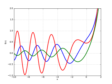
See coulombf() for additional information.

Plots

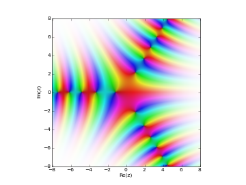
# Irregular Coulomb wave functions -- equivalent to figure 14.5 in A&S
F1 = lambda x: coulombg(0,0,x)
F2 = lambda x: coulombg(0,1,x)
F3 = lambda x: coulombg(0,5,x)
F4 = lambda x: coulombg(0,10,x)
F5 = lambda x: coulombg(0,x/2,x)
plot([F1,F2,F3,F4,F5], [0,30], [-2,2])

# Irregular Coulomb wave function in the complex plane
cplot(lambda z: coulombg(1,1,z), points=50000)

Examples

Evaluation is supported for arbitrary magnitudes of \(z\):

>>> from mpmath import *
>>> mp.dps = 25; mp.pretty = True
>>> coulombg(-2, 1.5, 3.5)
1.380011900612186346255524
>>> coulombg(2, 1.5, 3.5)
1.919153700722748795245926
>>> coulombg(-2, 1.5, '1e-10')
201126715824.7329115106793
>>> coulombg(-2, 1.5, 1000)
0.1802071520691149410425512
>>> coulombg(-2, 1.5, 10**10)
0.652103020061678070929794

The following reproduces a table in Abramowitz & Stegun, at twice the precision:

>>> mp.dps = 10
>>> eta = 2; z = 5
>>> for l in [1, 2, 3, 4, 5]:
...     print("%s %s %s" % (l, coulombg(l,eta,z),
...         -diff(lambda z: coulombg(l,eta,z), z)))
...
1 1.08148276 0.6028279961
2 1.496877075 0.5661803178
3 2.048694714 0.7959909551
4 3.09408669 1.731802374
5 5.629840456 4.549343289

Evaluation close to the singularity at \(z = 0\):

>>> mp.dps = 15
>>> coulombg(0,10,1)
3088184933.67358
>>> coulombg(0,10,'1e-10')
5554866000719.8
>>> coulombg(0,10,'1e-100')
5554866221524.1

Evaluation with a half-integer value for \(l\):

>>> coulombg(1.5, 1, 10)
0.852320038297334

coulombc()

mpmath.coulombc(l, eta)

Gives the normalizing Gamow constant for Coulomb wave functions,

\[C_l(\eta) = 2^l \exp\left(-\pi \eta/2 + [\ln \Gamma(1+l+i\eta) + \ln \Gamma(1+l-i\eta)]/2 - \ln \Gamma(2l+2)\right),\]

where the log gamma function with continuous imaginary part away from the negative half axis (see loggamma()) is implied.

This function is used internally for the calculation of Coulomb wave functions, and automatically cached to make multiple evaluations with fixed \(l\), \(\eta\) fast.

Confluent U and Whittaker functions

hyperu()

mpmath.hyperu(a, b, z)

Gives the Tricomi confluent hypergeometric function \(U\), also known as the Kummer or confluent hypergeometric function of the second kind. This function gives a second linearly independent solution to the confluent hypergeometric differential equation (the first is provided by \(\,_1F_1\) – see hyp1f1()).

Examples

Evaluation for arbitrary complex arguments:

>>> from mpmath import *
>>> mp.dps = 25; mp.pretty = True
>>> hyperu(2,3,4)
0.0625
>>> hyperu(0.25, 5, 1000)
0.1779949416140579573763523
>>> hyperu(0.25, 5, -1000)
(0.1256256609322773150118907 - 0.1256256609322773150118907j)

The \(U\) function may be singular at \(z = 0\):

>>> hyperu(1.5, 2, 0)
+inf
>>> hyperu(1.5, -2, 0)
0.1719434921288400112603671

Verifying the differential equation:

>>> a, b = 1.5, 2
>>> f = lambda z: hyperu(a,b,z)
>>> for z in [-10, 3, 3+4j]:
...     chop(z*diff(f,z,2) + (b-z)*diff(f,z) - a*f(z))
...
0.0
0.0
0.0

An integral representation:

>>> a,b,z = 2, 3.5, 4.25
>>> hyperu(a,b,z)
0.06674960718150520648014567
>>> quad(lambda t: exp(-z*t)*t**(a-1)*(1+t)**(b-a-1),[0,inf]) / gamma(a)
0.06674960718150520648014567

[1] http://people.math.sfu.ca/~cbm/aands/page_504.htm

whitm()

mpmath.whitm(k, m, z)

Evaluates the Whittaker function \(M(k,m,z)\), which gives a solution to the Whittaker differential equation

\[\frac{d^2f}{dz^2} + \left(-\frac{1}{4}+\frac{k}{z}+ \frac{(\frac{1}{4}-m^2)}{z^2}\right) f = 0.\]

A second solution is given by whitw().

The Whittaker functions are defined in Abramowitz & Stegun, section 13.1. They are alternate forms of the confluent hypergeometric functions \(\,_1F_1\) and \(U\):

\[ \begin{align}\begin{aligned}M(k,m,z) = e^{-\frac{1}{2}z} z^{\frac{1}{2}+m} \,_1F_1(\tfrac{1}{2}+m-k, 1+2m, z)\\W(k,m,z) = e^{-\frac{1}{2}z} z^{\frac{1}{2}+m} U(\tfrac{1}{2}+m-k, 1+2m, z).\end{aligned}\end{align} \]

Examples

Evaluation for arbitrary real and complex arguments is supported:

>>> from mpmath import *
>>> mp.dps = 25; mp.pretty = True
>>> whitm(1, 1, 1)
0.7302596799460411820509668
>>> whitm(1, 1, -1)
(0.0 - 1.417977827655098025684246j)
>>> whitm(j, j/2, 2+3j)
(3.245477713363581112736478 - 0.822879187542699127327782j)
>>> whitm(2, 3, 100000)
4.303985255686378497193063e+21707

Evaluation at zero:

>>> whitm(1,-1,0); whitm(1,-0.5,0); whitm(1,0,0)
+inf
nan
0.0

We can verify that whitm() numerically satisfies the differential equation for arbitrarily chosen values:

>>> k = mpf(0.25)
>>> m = mpf(1.5)
>>> f = lambda z: whitm(k,m,z)
>>> for z in [-1, 2.5, 3, 1+2j]:
...     chop(diff(f,z,2) + (-0.25 + k/z + (0.25-m**2)/z**2)*f(z))
...
0.0
0.0
0.0
0.0

An integral involving both whitm() and whitw(), verifying evaluation along the real axis:

>>> quad(lambda x: exp(-x)*whitm(3,2,x)*whitw(1,-2,x), [0,inf])
3.438869842576800225207341
>>> 128/(21*sqrt(pi))
3.438869842576800225207341

whitw()

mpmath.whitw(k, m, z)

Evaluates the Whittaker function \(W(k,m,z)\), which gives a second solution to the Whittaker differential equation. (See whitm().)

Examples

Evaluation for arbitrary real and complex arguments is supported:

>>> from mpmath import *
>>> mp.dps = 25; mp.pretty = True
>>> whitw(1, 1, 1)
1.19532063107581155661012
>>> whitw(1, 1, -1)
(-0.9424875979222187313924639 - 0.2607738054097702293308689j)
>>> whitw(j, j/2, 2+3j)
(0.1782899315111033879430369 - 0.01609578360403649340169406j)
>>> whitw(2, 3, 100000)
1.887705114889527446891274e-21705
>>> whitw(-1, -1, 100)
1.905250692824046162462058e-24

Evaluation at zero:

>>> for m in [-1, -0.5, 0, 0.5, 1]:
...     whitw(1, m, 0)
...
+inf
nan
0.0
nan
+inf

We can verify that whitw() numerically satisfies the differential equation for arbitrarily chosen values:

>>> k = mpf(0.25)
>>> m = mpf(1.5)
>>> f = lambda z: whitw(k,m,z)
>>> for z in [-1, 2.5, 3, 1+2j]:
...     chop(diff(f,z,2) + (-0.25 + k/z + (0.25-m**2)/z**2)*f(z))
...
0.0
0.0
0.0
0.0

Parabolic cylinder functions

pcfd()

mpmath.pcfd(n, z, **kwargs)

Gives the parabolic cylinder function in Whittaker’s notation \(D_n(z) = U(-n-1/2, z)\) (see pcfu()). It solves the differential equation

\[y'' + \left(n + \frac{1}{2} - \frac{1}{4} z^2\right) y = 0.\]

and can be represented in terms of Hermite polynomials (see hermite()) as

\[D_n(z) = 2^{-n/2} e^{-z^2/4} H_n\left(\frac{z}{\sqrt{2}}\right).\]

Plots

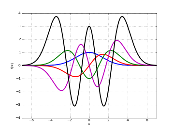
# Parabolic cylinder function D_n(x) on the real line for n=0,1,2,3,4
d0 = lambda x: pcfd(0,x)
d1 = lambda x: pcfd(1,x)
d2 = lambda x: pcfd(2,x)
d3 = lambda x: pcfd(3,x)
d4 = lambda x: pcfd(4,x)
plot([d0,d1,d2,d3,d4],[-7,7])

Examples

>>> from mpmath import *
>>> mp.dps = 25; mp.pretty = True
>>> pcfd(0,0); pcfd(1,0); pcfd(2,0); pcfd(3,0)
1.0
0.0
-1.0
0.0
>>> pcfd(4,0); pcfd(-3,0)
3.0
0.6266570686577501256039413
>>> pcfd('1/2', 2+3j)
(-5.363331161232920734849056 - 3.858877821790010714163487j)
>>> pcfd(2, -10)
1.374906442631438038871515e-9

Verifying the differential equation:

>>> n = mpf(2.5)
>>> y = lambda z: pcfd(n,z)
>>> z = 1.75
>>> chop(diff(y,z,2) + (n+0.5-0.25*z**2)*y(z))
0.0

Rational Taylor series expansion when \(n\) is an integer:

>>> taylor(lambda z: pcfd(5,z), 0, 7)
[0.0, 15.0, 0.0, -13.75, 0.0, 3.96875, 0.0, -0.6015625]

pcfu()

mpmath.pcfu(a, z, **kwargs)

Gives the parabolic cylinder function \(U(a,z)\), which may be defined for \(\Re(z) > 0\) in terms of the confluent U-function (see hyperu()) by

\[U(a,z) = 2^{-\frac{1}{4}-\frac{a}{2}} e^{-\frac{1}{4} z^2} U\left(\frac{a}{2}+\frac{1}{4}, \frac{1}{2}, \frac{1}{2}z^2\right)\]

or, for arbitrary \(z\),

\[e^{-\frac{1}{4}z^2} U(a,z) = U(a,0) \,_1F_1\left(-\tfrac{a}{2}+\tfrac{1}{4}; \tfrac{1}{2}; -\tfrac{1}{2}z^2\right) + U'(a,0) z \,_1F_1\left(-\tfrac{a}{2}+\tfrac{3}{4}; \tfrac{3}{2}; -\tfrac{1}{2}z^2\right).\]

Examples

Connection to other functions:

>>> from mpmath import *
>>> mp.dps = 25; mp.pretty = True
>>> z = mpf(3)
>>> pcfu(0.5,z)
0.03210358129311151450551963
>>> sqrt(pi/2)*exp(z**2/4)*erfc(z/sqrt(2))
0.03210358129311151450551963
>>> pcfu(0.5,-z)
23.75012332835297233711255
>>> sqrt(pi/2)*exp(z**2/4)*erfc(-z/sqrt(2))
23.75012332835297233711255
>>> pcfu(0.5,-z)
23.75012332835297233711255
>>> sqrt(pi/2)*exp(z**2/4)*erfc(-z/sqrt(2))
23.75012332835297233711255

pcfv()

mpmath.pcfv(a, z, **kwargs)

Gives the parabolic cylinder function \(V(a,z)\), which can be represented in terms of pcfu() as

\[V(a,z) = \frac{\Gamma(a+\tfrac{1}{2}) (U(a,-z)-\sin(\pi a) U(a,z)}{\pi}.\]

Examples

Wronskian relation between \(U\) and \(V\):

>>> from mpmath import *
>>> mp.dps = 25; mp.pretty = True
>>> a, z = 2, 3
>>> pcfu(a,z)*diff(pcfv,(a,z),(0,1))-diff(pcfu,(a,z),(0,1))*pcfv(a,z)
0.7978845608028653558798921
>>> sqrt(2/pi)
0.7978845608028653558798921
>>> a, z = 2.5, 3
>>> pcfu(a,z)*diff(pcfv,(a,z),(0,1))-diff(pcfu,(a,z),(0,1))*pcfv(a,z)
0.7978845608028653558798921
>>> a, z = 0.25, -1
>>> pcfu(a,z)*diff(pcfv,(a,z),(0,1))-diff(pcfu,(a,z),(0,1))*pcfv(a,z)
0.7978845608028653558798921
>>> a, z = 2+1j, 2+3j
>>> chop(pcfu(a,z)*diff(pcfv,(a,z),(0,1))-diff(pcfu,(a,z),(0,1))*pcfv(a,z))
0.7978845608028653558798921

pcfw()

mpmath.pcfw(a, z, **kwargs)

Gives the parabolic cylinder function \(W(a,z)\) defined in (DLMF 12.14).

Examples

Value at the origin:

>>> from mpmath import *
>>> mp.dps = 25; mp.pretty = True
>>> a = mpf(0.25)
>>> pcfw(a,0)
0.9722833245718180765617104
>>> power(2,-0.75)*sqrt(abs(gamma(0.25+0.5j*a)/gamma(0.75+0.5j*a)))
0.9722833245718180765617104
>>> diff(pcfw,(a,0),(0,1))
-0.5142533944210078966003624
>>> -power(2,-0.25)*sqrt(abs(gamma(0.75+0.5j*a)/gamma(0.25+0.5j*a)))
-0.5142533944210078966003624