Zeta functions, L-series and polylogarithms¶

This section includes the Riemann zeta functions and associated functions pertaining to analytic number theory.

Riemann and Hurwitz zeta functions¶

`zeta()`¶

mpmath.zeta(s, a=1, derivative=0)¶

Computes the Riemann zeta function

$\zeta(s) = 1+\frac{1}{2^s}+\frac{1}{3^s}+\frac{1}{4^s}+\ldots$

or, with $a \ne 1$ , the more general Hurwitz zeta function

$\zeta(s,a) = \sum_{k=0}^\infty \frac{1}{(a+k)^s}.$

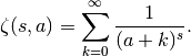
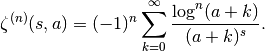
Optionally, zeta(s, a, n) computes the $n$ -th derivative with respect to $s$ ,

$\zeta^{(n)}(s,a) = (-1)^n \sum_{k=0}^\infty \frac{\log^n(a+k)}{(a+k)^s}.$

Although these series only converge for $\Re(s) > 1$ , the Riemann and Hurwitz zeta functions are defined through analytic continuation for arbitrary complex $s \ne 1$ ( $s = 1$ is a pole).

The implementation uses three algorithms: the Borwein algorithm for the Riemann zeta function when $s$ is close to the real line; the Riemann-Siegel formula for the Riemann zeta function when $s$ is large imaginary, and Euler-Maclaurin summation in all other cases. The reflection formula for $\Re(s) < 0$ is implemented in some cases. The algorithm can be chosen with method = 'borwein', method='riemann-siegel' or method = 'euler-maclaurin'.

The parameter $a$ is usually a rational number $a = p/q$ , and may be specified as such by passing an integer tuple $(p, q)$ . Evaluation is supported for arbitrary complex $a$ , but may be slow and/or inaccurate when $\Re(s) < 0$ for nonrational $a$ or when computing derivatives.

Examples

Some values of the Riemann zeta function:

>>> from mpmath import *
>>> mp.dps = 25; mp.pretty = True
>>> zeta(2); pi**2 / 6
1.644934066848226436472415
1.644934066848226436472415
>>> zeta(0)
-0.5
>>> zeta(-1)
-0.08333333333333333333333333
>>> zeta(-2)
0.0

For large positive $s$ , $\zeta(s)$ rapidly approaches 1:

>>> zeta(50)
1.000000000000000888178421
>>> zeta(100)
1.0
>>> zeta(inf)
1.0
>>> 1-sum((zeta(k)-1)/k for k in range(2,85)); +euler
0.5772156649015328606065121
0.5772156649015328606065121
>>> nsum(lambda k: zeta(k)-1, [2, inf])
1.0

Evaluation is supported for complex $s$ and $a$ :

>>> zeta(-3+4j)
(-0.03373057338827757067584698 + 0.2774499251557093745297677j)
>>> zeta(2+3j, -1+j)
(389.6841230140842816370741 + 295.2674610150305334025962j)

The Riemann zeta function has so-called nontrivial zeros on the critical line $s = 1/2 + it$ :

>>> findroot(zeta, 0.5+14j); zetazero(1)
(0.5 + 14.13472514173469379045725j)
(0.5 + 14.13472514173469379045725j)
>>> findroot(zeta, 0.5+21j); zetazero(2)
(0.5 + 21.02203963877155499262848j)
(0.5 + 21.02203963877155499262848j)
>>> findroot(zeta, 0.5+25j); zetazero(3)
(0.5 + 25.01085758014568876321379j)
(0.5 + 25.01085758014568876321379j)
>>> chop(zeta(zetazero(10)))
0.0

Evaluation on and near the critical line is supported for large heights $t$ by means of the Riemann-Siegel formula (currently for $a = 1$ , $n \le 4$ ):

>>> zeta(0.5+100000j)
(1.073032014857753132114076 + 5.780848544363503984261041j)
>>> zeta(0.75+1000000j)
(0.9535316058375145020351559 + 0.9525945894834273060175651j)
>>> zeta(0.5+10000000j)
(11.45804061057709254500227 - 8.643437226836021723818215j)
>>> zeta(0.5+100000000j, derivative=1)
(51.12433106710194942681869 + 43.87221167872304520599418j)
>>> zeta(0.5+100000000j, derivative=2)
(-444.2760822795430400549229 - 896.3789978119185981665403j)
>>> zeta(0.5+100000000j, derivative=3)
(3230.72682687670422215339 + 14374.36950073615897616781j)
>>> zeta(0.5+100000000j, derivative=4)
(-11967.35573095046402130602 - 218945.7817789262839266148j)
>>> zeta(1+10000000j)    # off the line
(2.859846483332530337008882 + 0.491808047480981808903986j)
>>> zeta(1+10000000j, derivative=1)
(-4.333835494679647915673205 - 0.08405337962602933636096103j)
>>> zeta(1+10000000j, derivative=4)
(453.2764822702057701894278 - 581.963625832768189140995j)

For investigation of the zeta function zeros, the Riemann-Siegel Z-function is often more convenient than working with the Riemann zeta function directly (see siegelz()).

Some values of the Hurwitz zeta function:

>>> zeta(2, 3); -5./4 + pi**2/6
0.3949340668482264364724152
0.3949340668482264364724152
>>> zeta(2, (3,4)); pi**2 - 8*catalan
2.541879647671606498397663
2.541879647671606498397663

For positive integer values of $s$ , the Hurwitz zeta function is equivalent to a polygamma function (except for a normalizing factor):

>>> zeta(4, (1,5)); psi(3, '1/5')/6
625.5408324774542966919938
625.5408324774542966919938

Evaluation of derivatives:

>>> zeta(0, 3+4j, 1); loggamma(3+4j) - ln(2*pi)/2
(-2.675565317808456852310934 + 4.742664438034657928194889j)
(-2.675565317808456852310934 + 4.742664438034657928194889j)
>>> zeta(2, 1, 20)
2432902008176640000.000242
>>> zeta(3+4j, 5.5+2j, 4)
(-0.140075548947797130681075 - 0.3109263360275413251313634j)
>>> zeta(0.5+100000j, 1, 4)
(-10407.16081931495861539236 + 13777.78669862804508537384j)
>>> zeta(-100+0.5j, (1,3), derivative=4)
(4.007180821099823942702249e+79 + 4.916117957092593868321778e+78j)

Generating a Taylor series at $s = 2$ using derivatives:

>>> for k in range(11): print("%s * (s-2)^%i" % (zeta(2,1,k)/fac(k), k))
...
1.644934066848226436472415 * (s-2)^0
-0.9375482543158437537025741 * (s-2)^1
0.9946401171494505117104293 * (s-2)^2
-1.000024300473840810940657 * (s-2)^3
1.000061933072352565457512 * (s-2)^4
-1.000006869443931806408941 * (s-2)^5
1.000000173233769531820592 * (s-2)^6
-0.9999999569989868493432399 * (s-2)^7
0.9999999937218844508684206 * (s-2)^8
-0.9999999996355013916608284 * (s-2)^9
1.000000000004610645020747 * (s-2)^10

Evaluation at zero and for negative integer $s$ :

>>> zeta(0, 10)
-9.5
>>> zeta(-2, (2,3)); mpf(1)/81
0.01234567901234567901234568
0.01234567901234567901234568
>>> zeta(-3+4j, (5,4))
(0.2899236037682695182085988 + 0.06561206166091757973112783j)
>>> zeta(-3.25, 1/pi)
-0.0005117269627574430494396877
>>> zeta(-3.5, pi, 1)
11.156360390440003294709
>>> zeta(-100.5, (8,3))
-4.68162300487989766727122e+77
>>> zeta(-10.5, (-8,3))
(-0.01521913704446246609237979 + 29907.72510874248161608216j)
>>> zeta(-1000.5, (-8,3))
(1.031911949062334538202567e+1770 + 1.519555750556794218804724e+426j)
>>> zeta(-1+j, 3+4j)
(-16.32988355630802510888631 - 22.17706465801374033261383j)
>>> zeta(-1+j, 3+4j, 2)
(32.48985276392056641594055 - 51.11604466157397267043655j)
>>> diff(lambda s: zeta(s, 3+4j), -1+j, 2)
(32.48985276392056641594055 - 51.11604466157397267043655j)

References

Dirichlet L-series¶

`altzeta()`¶

mpmath.altzeta(s)¶

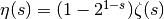
Gives the Dirichlet eta function, $\eta(s)$ , also known as the alternating zeta function. This function is defined in analogy with the Riemann zeta function as providing the sum of the alternating series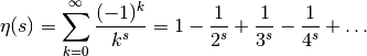

$\eta(s) = \sum_{k=0}^{\infty} \frac{(-1)^k}{k^s} = 1-\frac{1}{2^s}+\frac{1}{3^s}-\frac{1}{4^s}+\ldots$

The eta function, unlike the Riemann zeta function, is an entire function, having a finite value for all complex $s$ . The special case $\eta(1) = \log(2)$ gives the value of the alternating harmonic series.

The alternating zeta function may expressed using the Riemann zeta function as $\eta(s) = (1 - 2^{1-s}) \zeta(s)$ . It can also be expressed in terms of the Hurwitz zeta function, for example using dirichlet() (see documentation for that function).

Examples

Some special values are:

>>> from mpmath import *
>>> mp.dps = 15; mp.pretty = True
>>> altzeta(1)
0.693147180559945
>>> altzeta(0)
0.5
>>> altzeta(-1)
0.25
>>> altzeta(-2)
0.0

An example of a sum that can be computed more accurately and efficiently via altzeta() than via numerical summation:

>>> sum(-(-1)**n / mpf(n)**2.5 for n in range(1, 100))
0.867204951503984
>>> altzeta(2.5)
0.867199889012184

At positive even integers, the Dirichlet eta function evaluates to a rational multiple of a power of $\pi$ :

>>> altzeta(2)
0.822467033424113
>>> pi**2/12
0.822467033424113

Like the Riemann zeta function, $\eta(s)$ , approaches 1 as $s$ approaches positive infinity, although it does so from below rather than from above:

>>> altzeta(30)
0.999999999068682
>>> altzeta(inf)
1.0
>>> mp.pretty = False
>>> altzeta(1000, rounding='d')
mpf('0.99999999999999989')
>>> altzeta(1000, rounding='u')
mpf('1.0')

References

`dirichlet()`¶

mpmath.dirichlet(s, chi, derivative=0)¶

Evaluates the Dirichlet L-function

$L(s,\chi) = \sum_{k=1}^\infty \frac{\chi(k)}{k^s}.$

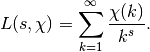
where $\chi$ is a periodic sequence of length $q$ which should be supplied in the form of a list $[\chi(0), \chi(1), \ldots, \chi(q-1)]$ . Strictly, $\chi$ should be a Dirichlet character, but any periodic sequence will work.

For example, dirichlet(s, [1]) gives the ordinary Riemann zeta function and dirichlet(s, [-1,1]) gives the alternating zeta function (Dirichlet eta function).

Also the derivative with respect to $s$ (currently only a first derivative) can be evaluated.

Examples

The ordinary Riemann zeta function:

>>> from mpmath import *
>>> mp.dps = 25; mp.pretty = True
>>> dirichlet(3, [1]); zeta(3)
1.202056903159594285399738
1.202056903159594285399738
>>> dirichlet(1, [1])
+inf

The alternating zeta function:

>>> dirichlet(1, [-1,1]); ln(2)
0.6931471805599453094172321
0.6931471805599453094172321

The following defines the Dirichlet beta function 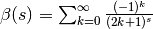$\beta(s) = \sum_{k=0}^\infty \frac{(-1)^k}{(2k+1)^s}$ and verifies several values of this function:

>>> B = lambda s, d=0: dirichlet(s, [0, 1, 0, -1], d)
>>> B(0); 1./2
0.5
0.5
>>> B(1); pi/4
0.7853981633974483096156609
0.7853981633974483096156609
>>> B(2); +catalan
0.9159655941772190150546035
0.9159655941772190150546035
>>> B(2,1); diff(B, 2)
0.08158073611659279510291217
0.08158073611659279510291217
>>> B(-1,1); 2*catalan/pi
0.5831218080616375602767689
0.5831218080616375602767689
>>> B(0,1); log(gamma(0.25)**2/(2*pi*sqrt(2)))
0.3915943927068367764719453
0.3915943927068367764719454
>>> B(1,1); 0.25*pi*(euler+2*ln2+3*ln(pi)-4*ln(gamma(0.25)))
0.1929013167969124293631898
0.1929013167969124293631898

A custom L-series of period 3:

>>> dirichlet(2, [2,0,1])
0.7059715047839078092146831
>>> 2*nsum(lambda k: (3*k)**-2, [1,inf]) + \
...   nsum(lambda k: (3*k+2)**-2, [0,inf])
0.7059715047839078092146831

Stieltjes constants¶

`stieltjes()`¶

mpmath.stieltjes(n, a=1)¶

For a nonnegative integer $n$ , stieltjes(n) computes the $n$ -th Stieltjes constant $\gamma_n$ , defined as the $n$ -th coefficient in the Laurent series expansion of the Riemann zeta function around the pole at $s = 1$ . That is, we have:

$\zeta(s) = \frac{1}{s-1} \sum_{n=0}^{\infty} \frac{(-1)^n}{n!} \gamma_n (s-1)^n$

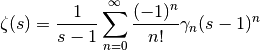
More generally, stieltjes(n, a) gives the corresponding coefficient $\gamma_n(a)$ for the Hurwitz zeta function $\zeta(s,a)$ (with $\gamma_n = \gamma_n(1)$ ).

Examples

The zeroth Stieltjes constant is just Euler’s constant $\gamma$ :

>>> from mpmath import *
>>> mp.dps = 15; mp.pretty = True
>>> stieltjes(0)
0.577215664901533

Some more values are:

>>> stieltjes(1)
-0.0728158454836767
>>> stieltjes(10)
0.000205332814909065
>>> stieltjes(30)
0.00355772885557316
>>> stieltjes(1000)
-1.57095384420474e+486
>>> stieltjes(2000)
2.680424678918e+1109
>>> stieltjes(1, 2.5)
-0.23747539175716

An alternative way to compute $\gamma_1$ :

>>> diff(extradps(15)(lambda x: 1/(x-1) - zeta(x)), 1)
-0.0728158454836767

stieltjes() supports arbitrary precision evaluation:

>>> mp.dps = 50
>>> stieltjes(2)
-0.0096903631928723184845303860352125293590658061013408

Algorithm

stieltjes() numerically evaluates the integral in the following representation due to Ainsworth, Howell and Coffey [1], [2]:

$\gamma_n(a) = \frac{\log^n a}{2a} - \frac{\log^{n+1}(a)}{n+1} + \frac{2}{a} \Re \int_0^{\infty} \frac{(x/a-i)\log^n(a-ix)}{(1+x^2/a^2)(e^{2\pi x}-1)} dx.$

For some reference values with $a = 1$ , see e.g. [4].

References

O. R. Ainsworth & L. W. Howell, “An integral representation of the generalized Euler-Mascheroni constants”, NASA Technical Paper 2456 (1985), http://ntrs.nasa.gov/archive/nasa/casi.ntrs.nasa.gov/19850014994_1985014994.pdf
M. W. Coffey, “The Stieltjes constants, their relation to the $\eta_j$ coefficients, and representation of the Hurwitz zeta function”, arXiv:0706.0343v1 http://arxiv.org/abs/0706.0343
http://mathworld.wolfram.com/StieltjesConstants.html
http://pi.lacim.uqam.ca/piDATA/stieltjesgamma.txt

Zeta function zeros¶

These functions are used for the study of the Riemann zeta function in the critical strip.

`zetazero()`¶

mpmath.zetazero(n, verbose=False)¶

Computes the $n$ -th nontrivial zero of $\zeta(s)$ on the critical line, i.e. returns an approximation of the $n$ -th largest complex number $s = \frac{1}{2} + ti$ for which $\zeta(s) = 0$ . Equivalently, the imaginary part $t$ is a zero of the Z-function (siegelz()).

Examples

The first few zeros:

>>> from mpmath import *
>>> mp.dps = 25; mp.pretty = True
>>> zetazero(1)
(0.5 + 14.13472514173469379045725j)
>>> zetazero(2)
(0.5 + 21.02203963877155499262848j)
>>> zetazero(20)
(0.5 + 77.14484006887480537268266j)

Verifying that the values are zeros:

>>> for n in range(1,5):
...     s = zetazero(n)
...     chop(zeta(s)), chop(siegelz(s.imag))
...
(0.0, 0.0)
(0.0, 0.0)
(0.0, 0.0)
(0.0, 0.0)

Negative indices give the conjugate zeros ( $n = 0$ is undefined):

>>> zetazero(-1)
(0.5 - 14.13472514173469379045725j)

zetazero() supports arbitrarily large $n$ and arbitrary precision:

>>> mp.dps = 15
>>> zetazero(1234567)
(0.5 + 727690.906948208j)
>>> mp.dps = 50
>>> zetazero(1234567)
(0.5 + 727690.9069482075392389420041147142092708393819935j)
>>> chop(zeta(_)/_)
0.0

with info=True, zetazero() gives additional information:

>>> mp.dps = 15
>>> zetazero(542964976,info=True)
((0.5 + 209039046.578535j), [542964969, 542964978], 6, '(013111110)')

This means that the zero is between Gram points 542964969 and 542964978; it is the 6-th zero between them. Finally (01311110) is the pattern of zeros in this interval. The numbers indicate the number of zeros in each Gram interval (Rosser blocks between parenthesis). In this case there is only one Rosser block of length nine.

`nzeros()`¶

mpmath.nzeros(t)¶

Computes the number of zeros of the Riemann zeta function in $(0,1) \times (0,t]$ , usually denoted by $N(t)$ .

Examples

The first zero has imaginary part between 14 and 15:

>>> from mpmath import *
>>> mp.dps = 15; mp.pretty = True
>>> nzeros(14)
0
>>> nzeros(15)
1
>>> zetazero(1)
(0.5 + 14.1347251417347j)

Some closely spaced zeros:

>>> nzeros(10**7)
21136125
>>> zetazero(21136125)
(0.5 + 9999999.32718175j)
>>> zetazero(21136126)
(0.5 + 10000000.2400236j)
>>> nzeros(545439823.215)
1500000001
>>> zetazero(1500000001)
(0.5 + 545439823.201985j)
>>> zetazero(1500000002)
(0.5 + 545439823.325697j)

This confirms the data given by J. van de Lune, H. J. J. te Riele and D. T. Winter in 1986.

`siegelz()`¶

mpmath.siegelz(t)¶

Computes the Z-function, also known as the Riemann-Siegel Z function,

$Z(t) = e^{i \theta(t)} \zeta(1/2+it)$

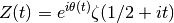
where $\zeta(s)$ is the Riemann zeta function (zeta()) and where $\theta(t)$ denotes the Riemann-Siegel theta function (see siegeltheta()).

Evaluation is supported for real and complex arguments:

>>> from mpmath import *
>>> mp.dps = 25; mp.pretty = True
>>> siegelz(1)
-0.7363054628673177346778998
>>> siegelz(3+4j)
(-0.1852895764366314976003936 - 0.2773099198055652246992479j)

The first four derivatives are supported, using the optional derivative keyword argument:

>>> siegelz(1234567, derivative=3)
56.89689348495089294249178
>>> diff(siegelz, 1234567, n=3)
56.89689348495089294249178

The Z-function has a Maclaurin expansion:

>>> nprint(chop(taylor(siegelz, 0, 4)))
[-1.46035, 0.0, 2.73588, 0.0, -8.39357]

The Z-function $Z(t)$ is equal to $\pm |\zeta(s)|$ on the critical line $s = 1/2+it$ (i.e. for real arguments $t$ to $Z$ ). Its zeros coincide with those of the Riemann zeta function:

>>> findroot(siegelz, 14)
14.13472514173469379045725
>>> findroot(siegelz, 20)
21.02203963877155499262848
>>> findroot(zeta, 0.5+14j)
(0.5 + 14.13472514173469379045725j)
>>> findroot(zeta, 0.5+20j)
(0.5 + 21.02203963877155499262848j)

Since the Z-function is real-valued on the critical line (and unlike $|\zeta(s)|$ analytic), it is useful for investigating the zeros of the Riemann zeta function. For example, one can use a root-finding algorithm based on sign changes:

>>> findroot(siegelz, [100, 200], solver='bisect')
176.4414342977104188888926

To locate roots, Gram points $g_n$ which can be computed by grampoint() are useful. If $(-1)^n Z(g_n)$ is positive for two consecutive $n$ , then $Z(t)$ must have a zero between those points:

>>> g10 = grampoint(10)
>>> g11 = grampoint(11)
>>> (-1)**10 * siegelz(g10) > 0
True
>>> (-1)**11 * siegelz(g11) > 0
True
>>> findroot(siegelz, [g10, g11], solver='bisect')
56.44624769706339480436776
>>> g10, g11
(54.67523744685325626632663, 57.54516517954725443703014)

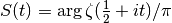
`siegeltheta()`¶

mpmath.siegeltheta(t)¶

Computes the Riemann-Siegel theta function,

$\theta(t) = \frac{ \log\Gamma\left(\frac{1+2it}{4}\right) - \log\Gamma\left(\frac{1-2it}{4}\right) }{2i} - \frac{\log \pi}{2} t.$

The Riemann-Siegel theta function is important in providing the phase factor for the Z-function (see siegelz()). Evaluation is supported for real and complex arguments:

>>> from mpmath import *
>>> mp.dps = 25; mp.pretty = True
>>> siegeltheta(0)
0.0
>>> siegeltheta(inf)
+inf
>>> siegeltheta(-inf)
-inf
>>> siegeltheta(1)
-1.767547952812290388302216
>>> siegeltheta(10+0.25j)
(-3.068638039426838572528867 + 0.05804937947429712998395177j)

Arbitrary derivatives may be computed with derivative = k

>>> siegeltheta(1234, derivative=2)
0.0004051864079114053109473741
>>> diff(siegeltheta, 1234, n=2)
0.0004051864079114053109473741

The Riemann-Siegel theta function has odd symmetry around $t = 0$ , two local extreme points and three real roots including 0 (located symmetrically):

>>> nprint(chop(taylor(siegeltheta, 0, 5)))
[0.0, -2.68609, 0.0, 2.69433, 0.0, -6.40218]
>>> findroot(diffun(siegeltheta), 7)
6.28983598883690277966509
>>> findroot(siegeltheta, 20)
17.84559954041086081682634

For large $t$ , there is a famous asymptotic formula for $\theta(t)$ , to first order given by:

>>> t = mpf(10**6)
>>> siegeltheta(t)
5488816.353078403444882823
>>> -t*log(2*pi/t)/2-t/2
5488816.745777464310273645

`grampoint()`¶

mpmath.grampoint(n)¶

Gives the $n$ -th Gram point $g_n$ , defined as the solution to the equation $\theta(g_n) = \pi n$ where $\theta(t)$ is the Riemann-Siegel theta function (siegeltheta()).

The first few Gram points are:

>>> from mpmath import *
>>> mp.dps = 25; mp.pretty = True
>>> grampoint(0)
17.84559954041086081682634
>>> grampoint(1)
23.17028270124630927899664
>>> grampoint(2)
27.67018221781633796093849
>>> grampoint(3)
31.71797995476405317955149

Checking the definition:

>>> siegeltheta(grampoint(3))
9.42477796076937971538793
>>> 3*pi
9.42477796076937971538793

A large Gram point:

>>> grampoint(10**10)
3293531632.728335454561153

Gram points are useful when studying the Z-function (siegelz()). See the documentation of that function for additional examples.

grampoint() can solve the defining equation for nonintegral $n$ . There is a fixed point where $g(x) = x$ :

>>> findroot(lambda x: grampoint(x) - x, 10000)
9146.698193171459265866198

References

http://mathworld.wolfram.com/GramPoint.html

`backlunds()`¶

mpmath.backlunds(t)¶

Computes the function $S(t) = \operatorname{arg} \zeta(\frac{1}{2} + it) / \pi$ .

See Titchmarsh Section 9.3 for details of the definition.

Examples

>>> from mpmath import *
>>> mp.dps = 15; mp.pretty = True
>>> backlunds(217.3)
0.16302205431184

Generally, the value is a small number. At Gram points it is an integer, frequently equal to 0:

>>> chop(backlunds(grampoint(200)))
0.0
>>> backlunds(extraprec(10)(grampoint)(211))
1.0
>>> backlunds(extraprec(10)(grampoint)(232))
-1.0

The number of zeros of the Riemann zeta function up to height $t$ satisfies $N(t) = \theta(t)/\pi + 1 + S(t)$ (see :func:nzeros` and siegeltheta()):

>>> t = 1234.55
>>> nzeros(t)
842
>>> siegeltheta(t)/pi+1+backlunds(t)
842.0

Lerch transcendent¶

`lerchphi()`¶

mpmath.lerchphi(z, s, a)¶

Gives the Lerch transcendent, defined for $|z| < 1$ and $\Re{a} > 0$ by

$\Phi(z,s,a) = \sum_{k=0}^{\infty} \frac{z^k}{(a+k)^s}$

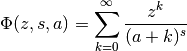
and generally by the recurrence $\Phi(z,s,a) = z \Phi(z,s,a+1) + a^{-s}$ along with the integral representation valid for $\Re{a} > 0$

$\Phi(z,s,a) = \frac{1}{2 a^s} + \int_0^{\infty} \frac{z^t}{(a+t)^s} dt - 2 \int_0^{\infty} \frac{\sin(t \log z - s \operatorname{arctan}(t/a)}{(a^2 + t^2)^{s/2} (e^{2 \pi t}-1)} dt.$

The Lerch transcendent generalizes the Hurwitz zeta function zeta() ( $z = 1$ ) and the polylogarithm polylog() ( $a = 1$ ).

Examples

Several evaluations in terms of simpler functions:

>>> from mpmath import *
>>> mp.dps = 25; mp.pretty = True
>>> lerchphi(-1,2,0.5); 4*catalan
3.663862376708876060218414
3.663862376708876060218414
>>> diff(lerchphi, (-1,-2,1), (0,1,0)); 7*zeta(3)/(4*pi**2)
0.2131391994087528954617607
0.2131391994087528954617607
>>> lerchphi(-4,1,1); log(5)/4
0.4023594781085250936501898
0.4023594781085250936501898
>>> lerchphi(-3+2j,1,0.5); 2*atanh(sqrt(-3+2j))/sqrt(-3+2j)
(1.142423447120257137774002 + 0.2118232380980201350495795j)
(1.142423447120257137774002 + 0.2118232380980201350495795j)

Evaluation works for complex arguments and $|z| \ge 1$ :

>>> lerchphi(1+2j, 3-j, 4+2j)
(0.002025009957009908600539469 + 0.003327897536813558807438089j)
>>> lerchphi(-2,2,-2.5)
-12.28676272353094275265944
>>> lerchphi(10,10,10)
(-4.462130727102185701817349e-11 + 1.575172198981096218823481e-12j)
>>> lerchphi(10,10,-10.5)
(112658784011940.5605789002 + 498113185.5756221777743631j)

Some degenerate cases:

>>> lerchphi(0,1,2)
0.5
>>> lerchphi(0,1,-2)
-0.5

Reduction to simpler functions:

>>> lerchphi(1, 4.25+1j, 1)
(1.044674457556746668033975 - 0.04674508654012658932271226j)
>>> zeta(4.25+1j)
(1.044674457556746668033975 - 0.04674508654012658932271226j)
>>> lerchphi(1 - 0.5**10, 4.25+1j, 1)
(1.044629338021507546737197 - 0.04667768813963388181708101j)
>>> lerchphi(3, 4, 1)
(1.249503297023366545192592 - 0.2314252413375664776474462j)
>>> polylog(4, 3) / 3
(1.249503297023366545192592 - 0.2314252413375664776474462j)
>>> lerchphi(3, 4, 1 - 0.5**10)
(1.253978063946663945672674 + 0.2316736622836535468765376j)

References

[DLMF] section 25.14

Polylogarithms and Clausen functions¶

`polylog()`¶

mpmath.polylog(s, z)¶

Computes the polylogarithm, defined by the sum

$\mathrm{Li}_s(z) = \sum_{k=1}^{\infty} \frac{z^k}{k^s}.$

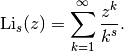
This series is convergent only for $|z| < 1$ , so elsewhere the analytic continuation is implied.

The polylogarithm should not be confused with the logarithmic integral (also denoted by Li or li), which is implemented as li().

Examples

The polylogarithm satisfies a huge number of functional identities. A sample of polylogarithm evaluations is shown below:

>>> from mpmath import *
>>> mp.dps = 15; mp.pretty = True
>>> polylog(1,0.5), log(2)
(0.693147180559945, 0.693147180559945)
>>> polylog(2,0.5), (pi**2-6*log(2)**2)/12
(0.582240526465012, 0.582240526465012)
>>> polylog(2,-phi), -log(phi)**2-pi**2/10
(-1.21852526068613, -1.21852526068613)
>>> polylog(3,0.5), 7*zeta(3)/8-pi**2*log(2)/12+log(2)**3/6
(0.53721319360804, 0.53721319360804)

polylog() can evaluate the analytic continuation of the polylogarithm when $s$ is an integer:

>>> polylog(2, 10)
(0.536301287357863 - 7.23378441241546j)
>>> polylog(2, -10)
-4.1982778868581
>>> polylog(2, 10j)
(-3.05968879432873 + 3.71678149306807j)
>>> polylog(-2, 10)
-0.150891632373114
>>> polylog(-2, -10)
0.067618332081142
>>> polylog(-2, 10j)
(0.0384353698579347 + 0.0912451798066779j)

Some more examples, with arguments on the unit circle (note that the series definition cannot be used for computation here):

>>> polylog(2,j)
(-0.205616758356028 + 0.915965594177219j)
>>> j*catalan-pi**2/48
(-0.205616758356028 + 0.915965594177219j)
>>> polylog(3,exp(2*pi*j/3))
(-0.534247512515375 + 0.765587078525922j)
>>> -4*zeta(3)/9 + 2*j*pi**3/81
(-0.534247512515375 + 0.765587078525921j)

Polylogarithms of different order are related by integration and differentiation:

>>> s, z = 3, 0.5
>>> polylog(s+1, z)
0.517479061673899
>>> quad(lambda t: polylog(s,t)/t, [0, z])
0.517479061673899
>>> z*diff(lambda t: polylog(s+2,t), z)
0.517479061673899

Taylor series expansions around $z = 0$ are:

>>> for n in range(-3, 4):
...     nprint(taylor(lambda x: polylog(n,x), 0, 5))
...
[0.0, 1.0, 8.0, 27.0, 64.0, 125.0]
[0.0, 1.0, 4.0, 9.0, 16.0, 25.0]
[0.0, 1.0, 2.0, 3.0, 4.0, 5.0]
[0.0, 1.0, 1.0, 1.0, 1.0, 1.0]
[0.0, 1.0, 0.5, 0.333333, 0.25, 0.2]
[0.0, 1.0, 0.25, 0.111111, 0.0625, 0.04]
[0.0, 1.0, 0.125, 0.037037, 0.015625, 0.008]

The series defining the polylogarithm is simultaneously a Taylor series and an L-series. For certain values of $z$ , the polylogarithm reduces to a pure zeta function:

>>> polylog(pi, 1), zeta(pi)
(1.17624173838258, 1.17624173838258)
>>> polylog(pi, -1), -altzeta(pi)
(-0.909670702980385, -0.909670702980385)

Evaluation for arbitrary, nonintegral $s$ is supported for $z$ within the unit circle:

>>> polylog(3+4j, 0.25)
(0.24258605789446 - 0.00222938275488344j)
>>> nsum(lambda k: 0.25**k / k**(3+4j), [1,inf])
(0.24258605789446 - 0.00222938275488344j)

It is also currently supported outside of the unit circle for $z$ not too large in magnitude:

>>> polylog(1+j, 20+40j)
(-7.1421172179728 - 3.92726697721369j)
>>> polylog(1+j, 200+400j)
Traceback (most recent call last):
  ...
NotImplementedError: polylog for arbitrary s and z

References

Richard Crandall, “Note on fast polylogarithm computation” http://people.reed.edu/~crandall/papers/Polylog.pdf
http://en.wikipedia.org/wiki/Polylogarithm
http://mathworld.wolfram.com/Polylogarithm.html

`clsin()`¶

mpmath.clsin(s, z)¶

Computes the Clausen sine function, defined formally by the series

$\mathrm{Cl}_s(z) = \sum_{k=1}^{\infty} \frac{\sin(kz)}{k^s}.$

The special case $\mathrm{Cl}_2(z)$ (i.e. clsin(2,z)) is the classical “Clausen function”. More generally, the Clausen function is defined for complex $s$ and $z$ , even when the series does not converge. The Clausen function is related to the polylogarithm (polylog()) as

$\mathrm{Cl}_s(z) = \frac{1}{2i}\left(\mathrm{Li}_s\left(e^{iz}\right) - \mathrm{Li}_s\left(e^{-iz}\right)\right) = \mathrm{Im}\left[\mathrm{Li}_s(e^{iz})\right] \quad (s, z \in \mathbb{R}),$

and this representation can be taken to provide the analytic continuation of the series. The complementary function clcos() gives the corresponding cosine sum.

Examples

Evaluation for arbitrarily chosen $s$ and $z$ :

>>> from mpmath import *
>>> mp.dps = 25; mp.pretty = True
>>> s, z = 3, 4
>>> clsin(s, z); nsum(lambda k: sin(z*k)/k**s, [1,inf])
-0.6533010136329338746275795
-0.6533010136329338746275795

Using $z + \pi$ instead of $z$ gives an alternating series:

>>> clsin(s, z+pi)
0.8860032351260589402871624
>>> nsum(lambda k: (-1)**k*sin(z*k)/k**s, [1,inf])
0.8860032351260589402871624

With $s = 1$ , the sum can be expressed in closed form using elementary functions:

>>> z = 1 + sqrt(3)
>>> clsin(1, z)
0.2047709230104579724675985
>>> chop((log(1-exp(-j*z)) - log(1-exp(j*z)))/(2*j))
0.2047709230104579724675985
>>> nsum(lambda k: sin(k*z)/k, [1,inf])
0.2047709230104579724675985

The classical Clausen function $\mathrm{Cl}_2(\theta)$ gives the value of the integral $\int_0^{\theta} -\ln(2\sin(x/2)) dx$ for $0 < \theta < 2 \pi$ :

>>> cl2 = lambda t: clsin(2, t)
>>> cl2(3.5)
-0.2465045302347694216534255
>>> -quad(lambda x: ln(2*sin(0.5*x)), [0, 3.5])
-0.2465045302347694216534255

This function is symmetric about $\theta = \pi$ with zeros and extreme points:

>>> cl2(0); cl2(pi/3); chop(cl2(pi)); cl2(5*pi/3); chop(cl2(2*pi))
0.0
1.014941606409653625021203
0.0
-1.014941606409653625021203
0.0

Catalan’s constant is a special value:

>>> cl2(pi/2)
0.9159655941772190150546035
>>> +catalan
0.9159655941772190150546035

The Clausen sine function can be expressed in closed form when $s$ is an odd integer (becoming zero when $s$ < 0):

>>> z = 1 + sqrt(2)
>>> clsin(1, z); (pi-z)/2
0.3636895456083490948304773
0.3636895456083490948304773
>>> clsin(3, z); pi**2/6*z - pi*z**2/4 + z**3/12
0.5661751584451144991707161
0.5661751584451144991707161
>>> clsin(-1, z)
0.0
>>> clsin(-3, z)
0.0

It can also be expressed in closed form for even integer $s \le 0$ , providing a finite sum for series such as $\sin(z) + \sin(2z) + \sin(3z) + \ldots$ :

>>> z = 1 + sqrt(2)
>>> clsin(0, z)
0.1903105029507513881275865
>>> cot(z/2)/2
0.1903105029507513881275865
>>> clsin(-2, z)
-0.1089406163841548817581392
>>> -cot(z/2)*csc(z/2)**2/4
-0.1089406163841548817581392

Call with pi=True to multiply $z$ by $\pi$ exactly:

>>> clsin(3, 3*pi)
-8.892316224968072424732898e-26
>>> clsin(3, 3, pi=True)
0.0

Evaluation for complex $s$ , $z$ in a nonconvergent case:

>>> s, z = -1-j, 1+2j
>>> clsin(s, z)
(-0.593079480117379002516034 + 0.9038644233367868273362446j)
>>> extraprec(20)(nsum)(lambda k: sin(k*z)/k**s, [1,inf])
(-0.593079480117379002516034 + 0.9038644233367868273362446j)

`clcos()`¶

mpmath.clcos(s, z)¶

Computes the Clausen cosine function, defined formally by the series

$\mathrm{\widetilde{Cl}}_s(z) = \sum_{k=1}^{\infty} \frac{\cos(kz)}{k^s}.$

This function is complementary to the Clausen sine function clsin(). In terms of the polylogarithm,

$\mathrm{\widetilde{Cl}}_s(z) = \frac{1}{2}\left(\mathrm{Li}_s\left(e^{iz}\right) + \mathrm{Li}_s\left(e^{-iz}\right)\right) = \mathrm{Re}\left[\mathrm{Li}_s(e^{iz})\right] \quad (s, z \in \mathbb{R}).$

Examples

Evaluation for arbitrarily chosen $s$ and $z$ :

>>> from mpmath import *
>>> mp.dps = 25; mp.pretty = True
>>> s, z = 3, 4
>>> clcos(s, z); nsum(lambda k: cos(z*k)/k**s, [1,inf])
-0.6518926267198991308332759
-0.6518926267198991308332759

Using $z + \pi$ instead of $z$ gives an alternating series:

>>> s, z = 3, 0.5
>>> clcos(s, z+pi)
-0.8155530586502260817855618
>>> nsum(lambda k: (-1)**k*cos(z*k)/k**s, [1,inf])
-0.8155530586502260817855618

With $s = 1$ , the sum can be expressed in closed form using elementary functions:

>>> z = 1 + sqrt(3)
>>> clcos(1, z)
-0.6720334373369714849797918
>>> chop(-0.5*(log(1-exp(j*z))+log(1-exp(-j*z))))
-0.6720334373369714849797918
>>> -log(abs(2*sin(0.5*z)))    # Equivalent to above when z is real
-0.6720334373369714849797918
>>> nsum(lambda k: cos(k*z)/k, [1,inf])
-0.6720334373369714849797918

It can also be expressed in closed form when $s$ is an even integer. For example,

>>> clcos(2,z)
-0.7805359025135583118863007
>>> pi**2/6 - pi*z/2 + z**2/4
-0.7805359025135583118863007

The case $s = 0$ gives the renormalized sum of $\cos(z) + \cos(2z) + \cos(3z) + \ldots$ (which happens to be the same for any value of $z$ ):

>>> clcos(0, z)
-0.5
>>> nsum(lambda k: cos(k*z), [1,inf])
-0.5

Also the sums

$\cos(z) + 2\cos(2z) + 3\cos(3z) + \ldots$

and

$\cos(z) + 2^n \cos(2z) + 3^n \cos(3z) + \ldots$

for higher integer powers $n = -s$ can be done in closed form. They are zero when $n$ is positive and even ( $s$ negative and even):

>>> clcos(-1, z); 1/(2*cos(z)-2)
-0.2607829375240542480694126
-0.2607829375240542480694126
>>> clcos(-3, z); (2+cos(z))*csc(z/2)**4/8
0.1472635054979944390848006
0.1472635054979944390848006
>>> clcos(-2, z); clcos(-4, z); clcos(-6, z)
0.0
0.0
0.0

With $z = \pi$ , the series reduces to that of the Riemann zeta function (more generally, if $z = p \pi/q$ , it is a finite sum over Hurwitz zeta function values):

>>> clcos(2.5, 0); zeta(2.5)
1.34148725725091717975677
1.34148725725091717975677
>>> clcos(2.5, pi); -altzeta(2.5)
-0.8671998890121841381913472
-0.8671998890121841381913472

Call with pi=True to multiply $z$ by $\pi$ exactly:

>>> clcos(-3, 2*pi)
2.997921055881167659267063e+102
>>> clcos(-3, 2, pi=True)
0.008333333333333333333333333

Evaluation for complex $s$ , $z$ in a nonconvergent case:

>>> s, z = -1-j, 1+2j
>>> clcos(s, z)
(0.9407430121562251476136807 + 0.715826296033590204557054j)
>>> extraprec(20)(nsum)(lambda k: cos(k*z)/k**s, [1,inf])
(0.9407430121562251476136807 + 0.715826296033590204557054j)

`polyexp()`¶

mpmath.polyexp(s, z)¶

Evaluates the polyexponential function, defined for arbitrary complex $s$ , $z$ by the series

$E_s(z) = \sum_{k=1}^{\infty} \frac{k^s}{k!} z^k.$

$E_s(z)$ is constructed from the exponential function analogously to how the polylogarithm is constructed from the ordinary logarithm; as a function of $s$ (with $z$ fixed), $E_s$ is an L-series It is an entire function of both $s$ and $z$ .

The polyexponential function provides a generalization of the Bell polynomials $B_n(x)$ (see bell()) to noninteger orders $n$ . In terms of the Bell polynomials,

$E_s(z) = e^z B_s(z) - \mathrm{sinc}(\pi s).$

Note that $B_n(x)$ and $e^{-x} E_n(x)$ are identical if $n$ is a nonzero integer, but not otherwise. In particular, they differ at $n = 0$ .

Examples

Evaluating a series:

>>> from mpmath import *
>>> mp.dps = 25; mp.pretty = True
>>> nsum(lambda k: sqrt(k)/fac(k), [1,inf])
2.101755547733791780315904
>>> polyexp(0.5,1)
2.101755547733791780315904

Evaluation for arbitrary arguments:

>>> polyexp(-3-4j, 2.5+2j)
(2.351660261190434618268706 + 1.202966666673054671364215j)

Evaluation is accurate for tiny function values:

>>> polyexp(4, -100)
3.499471750566824369520223e-36

If $n$ is a nonpositive integer, $E_n$ reduces to a special instance of the hypergeometric function $\,_pF_q$ :

>>> n = 3
>>> x = pi
>>> polyexp(-n,x)
4.042192318847986561771779
>>> x*hyper([1]*(n+1), [2]*(n+1), x)
4.042192318847986561771779

Zeta function variants¶

`primezeta()`¶

mpmath.primezeta(s)¶

Computes the prime zeta function, which is defined in analogy with the Riemann zeta function (zeta()) as

$P(s) = \sum_p \frac{1}{p^s}$

where the sum is taken over all prime numbers $p$ . Although this sum only converges for $\mathrm{Re}(s) > 1$ , the function is defined by analytic continuation in the half-plane $\mathrm{Re}(s) > 0$ .

Examples

Arbitrary-precision evaluation for real and complex arguments is supported:

>>> from mpmath import *
>>> mp.dps = 30; mp.pretty = True
>>> primezeta(2)
0.452247420041065498506543364832
>>> primezeta(pi)
0.15483752698840284272036497397
>>> mp.dps = 50
>>> primezeta(3)
0.17476263929944353642311331466570670097541212192615
>>> mp.dps = 20
>>> primezeta(3+4j)
(-0.12085382601645763295 - 0.013370403397787023602j)

The prime zeta function has a logarithmic pole at $s = 1$ , with residue equal to the difference of the Mertens and Euler constants:

>>> primezeta(1)
+inf
>>> extradps(25)(lambda x: primezeta(1+x)+log(x))(+eps)
-0.31571845205389007685
>>> mertens-euler
-0.31571845205389007685

The analytic continuation to $0 < \mathrm{Re}(s) \le 1$ is implemented. In this strip the function exhibits very complex behavior; on the unit interval, it has poles at $1/n$ for every squarefree integer $n$ :

>>> primezeta(0.5)         # Pole at s = 1/2
(-inf + 3.1415926535897932385j)
>>> primezeta(0.25)
(-1.0416106801757269036 + 0.52359877559829887308j)
>>> primezeta(0.5+10j)
(0.54892423556409790529 + 0.45626803423487934264j)

Although evaluation works in principle for any $\mathrm{Re}(s) > 0$ , it should be noted that the evaluation time increases exponentially as $s$ approaches the imaginary axis.

For large $\mathrm{Re}(s)$ , $P(s)$ is asymptotic to $2^{-s}$ :

>>> primezeta(inf)
0.0
>>> primezeta(10), mpf(2)**-10
(0.00099360357443698021786, 0.0009765625)
>>> primezeta(1000)
9.3326361850321887899e-302
>>> primezeta(1000+1000j)
(-3.8565440833654995949e-302 - 8.4985390447553234305e-302j)

References

Carl-Erik Froberg, “On the prime zeta function”, BIT 8 (1968), pp. 187-202.

`secondzeta()`¶

mpmath.secondzeta(s, a=0.015, **kwargs)¶

Evaluates the secondary zeta function $Z(s)$ , defined for $\mathrm{Re}(s)>1$ by

$Z(s) = \sum_{n=1}^{\infty} \frac{1}{\tau_n^s}$

where $\frac12+i\tau_n$ runs through the zeros of $\zeta(s)$ with imaginary part positive.

$Z(s)$ extends to a meromorphic function on $\mathbb{C}$ with a double pole at $s=1$ and simple poles at the points $-2n$ for $n=0$ , 1, 2, ...

Examples

>>> from mpmath import *
>>> mp.pretty = True; mp.dps = 15
>>> secondzeta(2)
0.023104993115419
>>> xi = lambda s: 0.5*s*(s-1)*pi**(-0.5*s)*gamma(0.5*s)*zeta(s)
>>> Xi = lambda t: xi(0.5+t*j)
>>> -0.5*diff(Xi,0,n=2)/Xi(0)
(0.023104993115419 + 0.0j)

We may ask for an approximate error value:

>>> secondzeta(0.5+100j, error=True)
((-0.216272011276718 - 0.844952708937228j), 2.22044604925031e-16)

The function has poles at the negative odd integers, and dyadic rational values at the negative even integers:

>>> mp.dps = 30
>>> secondzeta(-8)
-0.67236328125
>>> secondzeta(-7)
+inf

Implementation notes

The function is computed as sum of four terms $Z(s)=A(s)-P(s)+E(s)-S(s)$ respectively main, prime, exponential and singular terms. The main term $A(s)$ is computed from the zeros of zeta. The prime term depends on the von Mangoldt function. The singular term is responsible for the poles of the function.

The four terms depends on a small parameter $a$ . We may change the value of $a$ . Theoretically this has no effect on the sum of the four terms, but in practice may be important.

A smaller value of the parameter $a$ makes $A(s)$ depend on a smaller number of zeros of zeta, but $P(s)$ uses more values of von Mangoldt function.

We may also add a verbose option to obtain data about the values of the four terms.

>>> mp.dps = 10
>>> secondzeta(0.5 + 40j, error=True, verbose=True)
main term = (-30190318549.138656312556 - 13964804384.624622876523j)
    computed using 19 zeros of zeta
prime term = (132717176.89212754625045 + 188980555.17563978290601j)
    computed using 9 values of the von Mangoldt function
exponential term = (542447428666.07179812536 + 362434922978.80192435203j)
singular term = (512124392939.98154322355 + 348281138038.65531023921j)
((0.059471043 + 0.3463514534j), 1.455191523e-11)

>>> secondzeta(0.5 + 40j, a=0.04, error=True, verbose=True)
main term = (-151962888.19606243907725 - 217930683.90210294051982j)
    computed using 9 zeros of zeta
prime term = (2476659342.3038722372461 + 28711581821.921627163136j)
    computed using 37 values of the von Mangoldt function
exponential term = (178506047114.7838188264 + 819674143244.45677330576j)
singular term = (175877424884.22441310708 + 790744630738.28669174871j)
((0.059471043 + 0.3463514534j), 1.455191523e-11)

Notice the great cancellation between the four terms. Changing $a$ , the four terms are very different numbers but the cancellation gives the good value of Z(s).

References

A. Voros, Zeta functions for the Riemann zeros, Ann. Institute Fourier, 53, (2003) 665–699.

A. Voros, Zeta functions over Zeros of Zeta Functions, Lecture Notes of the Unione Matematica Italiana, Springer, 2009.

Zeta functions, L-series and polylogarithms¶

Riemann and Hurwitz zeta functions¶

`zeta()`¶

Dirichlet L-series¶

`altzeta()`¶

`dirichlet()`¶

Stieltjes constants¶

`stieltjes()`¶

Zeta function zeros¶

`zetazero()`¶

`nzeros()`¶

`siegelz()`¶

`siegeltheta()`¶

`grampoint()`¶

`backlunds()`¶

Lerch transcendent¶

`lerchphi()`¶

Polylogarithms and Clausen functions¶

`polylog()`¶

`clsin()`¶

`clcos()`¶

`polyexp()`¶

Zeta function variants¶

`primezeta()`¶

`secondzeta()`¶

Table Of Contents

Previous topic

Next topic

This Page

Navigation

Zeta functions, L-series and polylogarithms¶

Riemann and Hurwitz zeta functions¶

zeta()¶

Dirichlet L-series¶

altzeta()¶

dirichlet()¶

Stieltjes constants¶

stieltjes()¶

Zeta function zeros¶

zetazero()¶

nzeros()¶

siegelz()¶

siegeltheta()¶

grampoint()¶

backlunds()¶

Lerch transcendent¶

lerchphi()¶

Polylogarithms and Clausen functions¶

polylog()¶

clsin()¶

clcos()¶

polyexp()¶

Zeta function variants¶

primezeta()¶

secondzeta()¶

Table Of Contents

Previous topic

Next topic

This Page

Quick search

Navigation

`zeta()`¶

`altzeta()`¶

`dirichlet()`¶

`stieltjes()`¶

`zetazero()`¶

`nzeros()`¶

`siegelz()`¶

`siegeltheta()`¶

`grampoint()`¶

`backlunds()`¶

`lerchphi()`¶

`polylog()`¶

`clsin()`¶

`clcos()`¶

`polyexp()`¶

`primezeta()`¶

`secondzeta()`¶